Describing Data

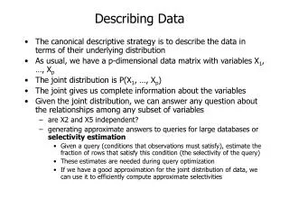
1. Describing Data • The canonical descriptive strategy is to describe the data in terms of their underlying distribution • As usual, we have a p-dimensional data matrix with variables X1, …, Xp • The joint distribution is P(X1, …, Xp) • The joint gives us complete information about the variables • Given the joint distribution, we can answer any question about the relationships among any subset of variables • are X2 and X5 independent? • generating approximate answers to queries for large databases or selectivity estimation • Given a query (conditions that observations must satisfy), estimate the fraction of rows that satisfy this condition (the selectivity of the query) • These estimates are needed during query optimization • If we have a good approximation for the joint distribution of data, we can use it to efficiently compute approximate selectivities

2. Graphical Models • In the next 3-4 lectures, we will be studying graphical models • e.g. Bayesian networks, Bayes nets, Belief nets, Markov networks, etc. • We will study: • representation • reasoning • learning • Materials based on upcoming book by Nir Friedman and Daphne Koller. Slides courtesy of Nir Friedman.

3. Probability Distributions • Let X1,…,Xp be random variables • Let P be a joint distribution over X1,…,Xp If the variables are binary, then we need O(2p) parameters to describe P Can we do better? • Key idea: use properties of independence

4. Independent Random Variables • Two variables X and Y are independent if • P(X = x|Y = y) = P(X = x) for all values x,y • That is, learning the values of Y does not change prediction of X • If X and Y are independent then • P(X,Y) = P(X|Y)P(Y) = P(X)P(Y) • In general, if X1,…,Xp are independent, then • P(X1,…,Xp)= P(X1)...P(Xp) • Requires O(n) parameters

5. Conditional Independence • Unfortunately, most of random variables of interest are not independent of each other • A more suitable notion is that of conditional independence • Two variables X and Y are conditionally independent given Z if • P(X = x|Y = y,Z=z) = P(X = x|Z=z) for all values x,y,z • That is, learning the values of Y does not change prediction of X once we know the value of Z • notation: I ( X , Y | Z )

6. Example: Naïve Bayesian Model • A common model in early diagnosis: • Symptoms are conditionally independent given the disease (or fault) • Thus, if • X1,…,Xp denote whether the symptoms exhibited by the patient (headache, high-fever, etc.) and • H denotes the hypothesis about the patients health • then, P(X1,…,Xp,H) = P(H)P(X1|H)…P(Xp|H), • This naïve Bayesian model allows compact representation • It does embody strong independence assumptions

7. Marge Homer Lisa Maggie Bart Example: Family trees Noisy stochastic process: Example: Pedigree • A node represents an individual’sgenotype • Modeling assumptions: • Ancestors can affect descendants' genotype only by passing genetic materials through intermediate generations

8. Y1 Y2 X Non-descendent Markov Assumption Ancestor • We now make this independence assumption more precise for directed acyclic graphs (DAGs) • Each random variable X, is independent of its non-descendents, given its parents Pa(X) • Formally,I (X, NonDesc(X) | Pa(X)) Parent Non-descendent Descendent

9. Burglary Earthquake Radio Alarm Call Markov Assumption Example • In this example: • I ( E, B ) • I ( B, {E, R} ) • I ( R, {A, B, C} | E ) • I ( A, R | B,E ) • I ( C, {B, E, R} | A)

10. X Y X Y I-Maps • A DAG G is an I-Map of a distribution P if all the Markov assumptions implied by G are satisfied by P (Assuming G and P both use the same set of random variables) Examples:

11. X Y Factorization • Given that G is an I-Map of P, can we simplify the representation of P? • Example: • Since I(X,Y), we have that P(X|Y) = P(X) • Applying the chain ruleP(X,Y) = P(X|Y) P(Y) = P(X) P(Y) • Thus, we have a simpler representation of P(X,Y)

12. Proof: • By chain rule: • wlog. X1,…,Xpis an ordering consistent with G • Hence, Factorization Theorem Thm: if G is an I-Map of P, then From assumption: • Since G is an I-Map, I (Xi, NonDesc(Xi)| Pa(Xi)) • We conclude, P(Xi | X1,…,Xi-1) = P(Xi | Pa(Xi) )

13. Burglary Earthquake Radio Alarm Call Factorization Example P(C,A,R,E,B) = P(B)P(E|B)P(R|E,B)P(A|R,B,E)P(C|A,R,B,E) versus P(C,A,R,E,B) = P(B) P(E) P(R|E) P(A|B,E) P(C|A)

14. Consequences • We can write P in terms of “local” conditional probabilities If G is sparse, • that is, |Pa(Xi)| < k ,  each conditional probability can be specified compactly • e.g. for binary variables, these require O(2k) params. representation of P is compact • linear in number of variables

15. Pause…Summary We defined the following concepts • The Markov Independences of a DAG G • I (Xi , NonDesc(Xi) | Pai ) • G is an I-Map of a distribution P • If P satisfies the Markov independencies implied by G We proved the factorization theorem • if G is an I-Map of P, then

16. Conditional Independencies • Let Markov(G) be the set of Markov Independencies implied by G • The factorization theorem shows G is an I-Map of P  • We can also show the opposite: Thm:  Gis an I-Map of P

17. Proof (Outline) Example: X Z Y

18. Implied Independencies • Does a graph G imply additional independencies as a consequence of Markov(G)? • We can define a logic of independence statements • Some axioms: • I( X ; Y | Z )  I( Y; X | Z ) • I( X ; Y1, Y2 | Z )  I( X; Y1 | Z )

19. d-seperation • A procedure d-sep(X; Y | Z, G) that given a DAG G, and sets X, Y, and Z returns either yes or no • Goal: d-sep(X; Y | Z, G) = yes iff I(X;Y|Z) follows from Markov(G)

20. Burglary Earthquake Radio Alarm Call Paths • Intuition: dependency must “flow” along paths in the graph • A path is a sequence of neighboring variables Examples: • R  E  A  B • C A E  R

21. Paths • We want to know when a path is • active -- creates dependency between end nodes • blocked -- cannot create dependency end nodes • We want to classify situations in which paths are active.

22. E E Blocked Blocked Unblocked Active R R A A Path Blockage Three cases: • Common cause

23. Blocked Blocked Unblocked Active E E A A C C Path Blockage Three cases: • Common cause • Intermediate cause

24. Blocked Blocked Unblocked Active E E E B B B A A A C C C Path Blockage Three cases: • Common cause • Intermediate cause • Common Effect

25. Path Blockage -- General Case A path is active, given evidence Z, if • Whenever we have the configurationB or one of its descendents are in Z • No other nodes in the path are in Z A path is blocked, given evidence Z, if it is not active. A C B

26. d-sep(R,B)? Example E B R A C

27. d-sep(R,B) = yes d-sep(R,B|A)? Example E B R A C

28. d-sep(R,B) = yes d-sep(R,B|A) = no d-sep(R,B|E,A)? Example E B R A C

29. d-Separation • X is d-separated from Y, given Z, if all paths from a node in X to a node in Y are blocked, given Z. • Checking d-separation can be done efficiently (linear time in number of edges) • Bottom-up phase: Mark all nodes whose descendents are in Z • X to Y phase:Traverse (BFS) all edges on paths from X to Y and check if they are blocked

30. Soundness Thm: • If • G is an I-Map of P • d-sep( X; Y | Z, G ) = yes • then • P satisfies I( X; Y | Z ) Informally, • Any independence reported by d-separation is satisfied by underlying distribution

31. Completeness Thm: • If d-sep( X; Y | Z, G ) = no • then there is a distribution P such that • G is an I-Map of P • P does not satisfy I( X; Y | Z ) Informally, • Any independence not reported by d-separation might be violated by the underlying distribution • We cannot determine this by examining the graph structure alone

32. X2 X1 X2 X1 X3 X4 X3 X4 I-Maps revisited • The fact that G is I-Map of P might not be that useful • For example, complete DAGs • A DAG is G is complete if we cannot add an arc without creating a cycle • These DAGs do not imply any independencies • Thus, they are I-Maps of any distribution

33. Minimal I-Maps A DAG G is a minimal I-Map of P if • G is an I-Map of P • If G’  G, then G’ is not an I-Map of P Removing any arc from G introduces (conditional) independencies that do not hold in P

34. X2 X1 X3 X4 X2 X1 X3 X4 X2 X1 X2 X1 X2 X1 X3 X4 X3 X4 X3 X4 Minimal I-Map Example • If is a minimal I-Map • Then, these are not I-Maps:

35. Constructing minimal I-Maps The factorization theorem suggests an algorithm • Fix an ordering X1,…,Xn • For each i, • select Pai to be a minimal subset of {X1,…,Xi-1 },such that I(Xi ; {X1,…,Xi-1 } - Pai | Pai ) • Clearly, the resulting graph is a minimal I-Map.

36. E B E B R A R A C C Non-uniqueness of minimal I-Map • Unfortunately, there may be several minimal I-Maps for the same distribution • Applying I-Map construction procedure with different orders can lead to different structures Order:C, R, A, E, B Original I-Map

37. Choosing Ordering & Causality • The choice of order can have drastic impact on the complexity of minimal I-Map • Heuristic argument: construct I-Map using causal ordering among variables • Justification? • It is often reasonable to assume that graphs of causal influence should satisfy the Markov properties.

38. P-Maps • A DAG G is P-Map (perfect map) of a distribution P if • I(X; Y | Z) if and only if d-sep(X; Y |Z, G) = yes Notes: • A P-Map captures all the independencies in the distribution • P-Maps are unique, up to DAG equivalence

39. P-Maps • Unfortunately, some distributions do not have a P-Map • Example: • A minimal I-Map: • This is not a P-Map since I(A;C) but d-sep(A;C) = no A B C

40. Bayesian Networks • A Bayesian network specifies a probability distribution via two components: • A DAG G • A collection of conditional probability distributions P(Xi|Pai) • The joint distribution P is defined by the factorization • Additional requirement: G is a minimal I-Map of P

41. Summary • We explored DAGs as a representation of conditional independencies: • Markov independencies of a DAG • Tight correspondence between Markov(G) and the factorization defined by G • d-separation, a sound & complete procedure for computing the consequences of the independencies • Notion of minimal I-Map • P-Maps • This theory is the basis for defining Bayesian networks

42. Markov Networks • We now briefly consider an alternative representation of conditional independencies • Let U be an undirected graph • Let Ni be the set of neighbors of Xi • Define Markov(U) to be the set of independenciesI( Xi ; {X1,…,Xn} - Ni - {Xi } | Ni ) • U is an I-Map of P if P satisfies Markov(U)

43. Example This graph implies that • I(A; C | B, D ) • I(B; D | A, C ) • Note: this example does not have a directed P-Map B A D C

44. Markov Network Factorization Thm: if • P is strictly positive, that is P(x1, …, xn )> 0 for all assignments then • U is an I-Map of P if and only if • there is a factorization where C1, …, Ck are the maximal cliques in U Alternative form:

45. Relationship between Directed & Undirected Models Chain Graphs Directed Graphs Undirected Graphs

46. CPDs • So far, we focused on how to represent independencies using DAGs • The “other” component of a Bayesian networks is the specification of the conditional probability distributions (CPDs) • We start with the simplest representation of CPDs and then discuss additional structure

47. A 0 0 1 1 B 0 0 1 1 P(C = 0 | A, B) 0.25 0.33 0.50 0.12 P(C = 1 | A, B) 0.88 0.50 0.75 0.67 Tabular CPDs • When the variable of interest are all discrete, the common representation is as a table: • For example P(C|A,B) can be represented by

48. Tabular CPDs Pros: • Very flexible, can capture any CPD of discrete variables • Can be easily stored and manipulated Cons: • Representation size grows exponentially with the number of parents! • Unwieldy to assess probabilities for more than few parents

49. Structured CPD • To avoid the exponential blowup in representation, we need to focus on specialized types of CPDs • This comes at a cost in terms of expressive power • We now consider several types of structured CPDs

50. Disease 2 Disease 3 Disease 1 Fever Causal Independence • Consider the following situation • In tabular CPD, we need to assess the probability of fever in eight cases • These involve all possible interactions between diseases • For three disease, this might be feasible….For ten diseases, not likely….