Download

1 / 29
330 likes | 697 Views
INTRODUCTION TO AN ALYSIS O F VA RIANCE (ANOVA). COURSE CONTENT. WHAT IS ANOVA DIFFERENT TYPES OF ANOVA ANOVA THEORY WORKED EXAMPLE IN EXCEL GENERATING THE DATA EXPLANATION/INTERPRETATION OF OUTPUT RULES FOR ACCEPTING/REJECTING NULL HYPOTHESIS SUPPLEMENTAL TESTING

E N D
COURSE CONTENT • WHAT IS ANOVA • DIFFERENT TYPES OF ANOVA • ANOVA THEORY • WORKED EXAMPLE IN EXCEL • GENERATING THE DATA • EXPLANATION/INTERPRETATION OF OUTPUT • RULES FOR ACCEPTING/REJECTING NULL HYPOTHESIS • SUPPLEMENTAL TESTING • SUMMARY – ANOVA IN EXCEL • SUMMARY
WHAT IS ANOVA? The t-test is designed to test the hypothesis that 2 means could be from the same population data. But what if we want to compare more than 2 means at the same time? ANOVA is a general technique that can be used to test the hypothesis that the means among two or more groups are equal, (under the assumption that the sampled populations are normally distribute.) ANOVA can be used to test differences among several means for significance without increasing the Type 1 error rate.
DIFFERENT TYPES OF ANOVA • To begin, let us consider the effect of temperature on a passive component such as a resistor. • We select three different temperatures and observe their effect on the resistors. • The experiment can be conducted by measuring all the participating resistors before placing n resistors each in three different ovens. • Each oven is heated to a selected temperature. Then we measure the resistors again after, say, 24 hours and analyze the responses, which are the difference between before and after being subjected to the temperatures. • The temperature is called a factor. • The different temperature settings are called levels. In this example there are three levels or settings of the factor temperature.
ANOVA THEORY • The theory of ANOVA is long, complicated and detailed and will NOT be looked at in this course. • If you do want to learn more, try the following web pages: • http://davidmlane.com/hyperstat/intro_ANOVA.html • http://itl.nist.gov/div898/handbook/prc/section4/prc43.htm • http://www.experiment-resources.com/anova-test.html • http://www.chem.agilent.com/cag/bsp/products/gsgx/Downloads/pdf/org
A WORKED EXAMPLE • In this example of a one way ANOVA we will calculate all the components of the AVOVA without explaining the theory behind the formulas used. • The main objectives of this exercise are to learn about the typical layout of ANOVA output (the format will look very siilar in excel) and to learn how to interpret the output. • And finally how to carry out ANOVA using excel.
In a hypothetical experiment, aspirin, Tylenol and placebo were tested to see how much pain relief each provides. • Pain relief was rated on a five-point scale. Four subjects were tested in each group and their data are shown below: How many factors? How many subject in total? How many levels?
A WORKED EXAMPLE Interpretation of output
Now we have an output – we can deconstruct each result and explain the final result.
Total Sum of Squares The variation among all the subjects in an experiment is measured by what is called total sum of square or SST. SST is the sum of the squared differences of each score from the mean of all scores, then SST = Ʃ[X – GM]² Where GM = ƩX/N and N is the total number of subjects in the experiment.
For the example data: N = 12 GM = [3+5+3+5+2+2+4+4+2+1+3+2] / 12 = ??? SST = [3-3]²+[5-3]²+[3-3] ²+[5-3] ²+[2-3] ²+[2-3] ² +[4-3] ²+[4-3] ²+[2-3] ²+[1-3] ²+[3-3] ²+[2-3] ² = ???
Mean squares are estimates of variance and are computed by dividing the sum of squares by the degrees of freedom. The mean square for groups [4.00] was computed by dividing the sum of squares for groups [8.00] by the degrees of freedom for groups [2].
The F ratio is computed by dividing the mean square for between groups by the mean square for between groups by the mean square for within groups. In this example, F = 4 / 1.111 = 3.6
The probability value it is the probability of the obtaining an F as large or lager than the one computed in the data assuming that the null hypothesis is true. It can be computed from an F table. The df for groups [2] is used as the degrees of freedom in the numerator and the df for error [9] is used as the degrees of freedom in the denominator. The probability of an F with 2 and 9 df as larger or larger than 3.60 is 0.07. F crit is the hingest value of F that can be obtained without rejecting the null hypothesis (obtained from F-test tables for 2 & 9 DF)
Interpreting the ANOVA One Way test results. Using the above table and the results from the example is there an indication of a significant difference in the means.
Unfortunately, when the analysis of variance is significant and the null hypothesis is rejected, • The only valid inference that can be made is that at least one population mean is different from at least one other population mean. • The analysis of variance does not reveal which population means differ from which others. Consequently, further analysis are usually conducted after a significant analysis of variance. These further analysis almost always involve conducting a series of significance tests.
SUMMARY ANOVA: Single Factor • This tool performs a simple analysis of variance on data for two or more samples. • The analysis provides a test of the hypothesis that each sample is drawn from the same underlying probability distribution against the alternative hypothesis that underlying probability distributions are not the same for all samples. • If there are only two samples, you can use the worksheet function T-TEST. • With more than two samples, there is no convenient generalization of T-TEST, and the single factor ANOVA model can be called upon instead.
SUMMARY ANOVA: Two Factor with Replication • This analysis tool is useful when data can be classified along two different dimensions. • For example, in an experiment to measure the height of plants, the plants may be given different brands of fertilizer (i.e: A,B,C) and might also be kept at different temperature (i.e: low, high). • For each of the six possible pairs of (fertilizer, temperature), we have an equal number of observations of plant height. • Using this ANOVA tool, we can test: • Whether the heights of plants for the different fertilizer brands are drawn from the same underlying population. Temperatures are ignored for this analysis. • Whether the heights of plants for the different temperature levels are drawn from the same underlying population. Fertilizer brands are ignored for this analysis.
SUMMARY • Whether, having accounted for the effects of differences between fertilizer brands found in the first bulleted point, and differences in temperatures found in the second bulleted point, the six samples representing all pairs of (fertilizer, temperature) values are drawn from the same population. • The alternative hypothesis is that there are affects due to specific (fertilizer, temperature) pairs over and above the differences that are based on fertilizer alone or on temperature alone.
SUMMARY ANOVA: Two Factor Without Replication • This analysis tool is useful when data is classified on two different dimensions as in the Two-Factor case with replication. • However, for this tool it is assumed that there is only a single observation for each pair (for example, each {fertilizer, temperature} pair in the preceding example).
Summary • To compare 2 or more means in a single test we use ANOVA. • The type of ANOVA test to use is decided by the number of FACTORS in the experiment. • The ANOVA only tell whether there is a significant difference and gives no information on which mean(s) are different.