Introduction to Factorial ANOVA Designs
370 likes | 536 Views
Factorial ANOVA is a statistical method used to analyze the effects of multiple independent variables (IVs) on a dependent variable (DV). It can involve two-way, three-way, or even more complex designs, focusing on interactions between factors. Key components include main effects, interaction effects, and variability sources. This guide covers calculations of sums of squares, degrees of freedom, and effect sizes, and emphasizes the significance of interactions in interpreting results. Graphical representations of interactions enhance understanding. Ensure results are interpreted within theoretical contexts.

Introduction to Factorial ANOVA Designs
E N D
Presentation Transcript
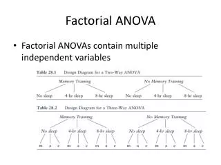
Factorial Anova • With factorial Anova we have more than one independent variable • The terms 2-way, 3-way etc. refer to how many IVs there are in the analysis • The following will discuss 2-way design but may extended to more complex designs. • The analysis of interactions constitutes the focal point of factorial design
Recall the one-way Anova • Total variability comes from: • Differences between groups • Differences within groups
Factorial Anova • With factorial designs we have additional sources of variability to consider • Main effects • Mean differences among the levels of a particular factor • Interaction • Differences among cell means not attributable to main effects • When the effect of one factor is influenced by the levels of another
Total variability Between-treatments var. Within-treatments var. Interaction variability Factor A variability Factor B variability Partition of Variability
Example: • Arousal, task difficulty and performance • Yerkes-Dodson
Example • SStotal = ∑(X – grand mean)2 • SStotal = 360 • Df = N – 1 = 29 • SSb/t =∑n(cell means – grand mean)2 • = 5(3-4)2 + … 5(1-4)2 • SSb/t =240 • Df= K# of cells – 1 = 5 • SSw/in = ∑(X – respective cell means)2 or SStotal- SSb/t • SSw/in = 120 • Df = N-K = 24
Sums of Squares Between • SSDifficulty = n(row means –grand mean)2 • = 15(6-4)2 + 15(2-4)2 = 120 • Df = # of rows (levels) – 1 = 1 • SSArousal = n(col means – grand mean)2 • = 10(2-4)2 + 10(5-4)2 + 10(5-4)2 = 60 • Df = # of columns (levels) – 1 = 2 • SSDXA = SSb/t - SSDifficulty - SSArousal • = 240 - 120 - 60 = 60 • Df = dfb/t - dfDifficulty – dfArousal = 5-1-2 = 2 • Or dfdiff X dfarous
Output • Mean squares and F-statistics are calculated as before
Initial Interpretation • Significant main effects of task difficulty and arousal level, as well as a significant interaction • Difficulty • Better performance for easy items • Arousal • Low worst • Interaction • Easy better in general but much more so with high arousal
Eta-squared is given as the effect size for B/t groups (SSeffect/SStotal) • Partial eta-squared is given for the remaining factors: SSeffect/(SSeffect + SSerror) • End result: significance w/ large effect sizes
Graphical display of interactions • Two ways to display previous results
No interaction Interaction Graphical display of interactions • What are we looking for? • Do the lines behave similarly (are parallel) or not? • Does the effect of one factor depend on the level of the other factor?
The general linear model • Recall for the general one-way anova • Where: • μ = grand mean • = effect of Treatment A (μa – μ) • ε = within cell error • So a person’s score is a function of the grand mean, the treatment mean, and within cell error
Effects for 2-way Population main effect associated with the treatment Aj (first factor): Population main effect associated with treatment Bk (second factor): The interaction is defined as , the joint effect of treatment levels j and k (interaction of and ) so the linear model is: Each person’s score is a function of the grand mean, the treatment means, and their interaction (plus w/in cell error).
The general linear model • The interaction is a residual: • Plugging in and leads to:
Partitioning of total sum of squares • Squaring yields • Interaction sum of squares can be obtained as remainder
Partitioning of total sum of squares • SSA: factor A sum of squares measures the variability of the estimated factor A level means • The more variable they are, the bigger will be SSA • Likewise for SSB • SSAB is the AB interaction sum of squares and measures the variability of the estimated interactions
GLM Factorial ANOVA Statistical Model: Statistical Hypothesis: The interaction null is that the cell means do not differ significantly (from the grand mean) outside of the main effects present, i.e. that this residual effect is zero
Interpretation: sig main fx and interaction • Note that with a significant interaction, the main effects are understood only in terms of that interaction • In other words, they cannot stand alone as an explanation and must be qualified by the interaction’s interpretation • Some take issue with even talking about the main effects, but noting them initially may make the interaction easier for others to understand when you get to it
Interpretation: sig main fx and interaction • However, interpretation depends on common sense, and should adhere to theoretical considerations • Plot your results in different ways • If main effects are meaningful, then it makes sense to talk about them, whether or not an interaction is statistically significant or not • E.g. note that there is a gender effect but w/ interaction we now see that it is only for level(s) X of Factor B • To help you interpret results, test simple effects • Is simple effect of A significant within specific levels of B? • Is simple effect of B significant within specific levels of A?
Simple effects • Analysis of the effects of one factor at one level of the other factor • Some possibilities from previous example • Arousal for easy items (or hard items) • Difficulty for high arousal condition (or medium or low)
Simple effects • SSarousal for easy items= 5(3-6)2 + 5(6-6)2 + 5(9-6)2 = 90 • SSarousal for difficult items= 5(1-2)2 + 5(4-2)2 + 5(1-2)2 = 30 • SSdifficulty at lo = 5(3-2)2 + 5(1-2)2 = 10 • SSdifficulty at med= 5(6-5)2 + 5(4-5)2 = 10 • SSdifficulty at hi= 5(9-5)2 + 5(1-5)2 = 160
Simple effects • Note that the simple effect represents a partitioning of SSmain effect and SSinteraction • NOT JUST THE INTERACTION!! • From Anova table: • SSarousal + SSarousal by difficulty = 60 + 60 = 120 • SSarousal for easy items= 90 • SSarousal for difficult items= 30 • 90 + 30 = 120 • SSdifficulty + SSarousal by difficulty = 120 + 60 = 180 • SSdifficulty at lo = 10 • SSdifficulty at med= 10 • SSdifficulty at hi= 160 • 10 + 10 + 160 = 180
Pulling it off in SPSS Paste!
Pulling it off in SPSS • Add • /EMMEANS = tables(a*b)compare(a) • /EMMEANS = tables(a*b)compare(b)
Pulling it off in SPSS • Output
Test for simple fx with no sig interaction? • What if there was no significant interaction, do I still test for simple effects? • Maybe, but more on that later • A significant simple effect suggests that at least one of the slopes across levels is significantly different than zero • However, one would not conclude that the interaction is ‘close enough’ just because there was a significant simple effect • The nonsig interaction suggests that the slope seen is not statistically different from the other(s) under consideration.
Multiple comparisons and contrasts • For main effects multiple comparisons and contrasts can be conducted as would be normally • One would have all the same considerations for choosing a particular method of post hoc analysis or weights for contrast analysis
Multiple comparisons and contrasts • With interactions post hocs can be run comparing individual cell means • The problem is that it rarely makes theoretical sense to compare many of the pairs of means under consideration
Contrasts for interactions • We may have a specific result to look for with regard to our interaction • For example, we may think based on past research moderate arousal should result in optimal performance for difficult items • We would assign contrast weights to reflect this hypothesis
Analyze General Linear Model Univariate Select Dependent Variable and Specify Fixed and/or Random Factor(s) (Treatment Groups and or Patient Characteristic(s), Treatment Sites, etc.) Paste Launches Syntax Window Add /LMATRIX command lines RUN All Pulling it off in SPSS
/LMATRIX Command /LMATRIX ‘<Title for 1st Contrast>’ <Specify Weights for 1st Contrast>; ‘<Title for 2nd Contrast>’ <Specify Weights for 2nd Contrast>; … ‘<Title for Final Contrast>’ <Specify Weights for Final Contrast>
For this 3 X 2 design the weights will order as follows: • A1B1 A1B2 A2B1 A2B2 A3B1 A3B2 • Note for this example, SPSS is analyzing categories in alphabetical order • Arousal hi lo med • Task Diff Easy • In other words • Hi:Difficult Hi:Easy Lo:Difficult … Med:Easy
As alluded to previously it is possible to have: • Sig overall F • Sig contrast • Nonsig posthoc • Nonsig F • Nonsig contrast • e.g. 1 & 3 VS. 2 • Sig posthoc • 1 vs. 2 sig
A different model ☺ • If cognitive anxiety is low, then the performance effects of physiological arousal will be low; but if it is high, the effects will be large and sudden.