Chapter V. Amplitude Modulations
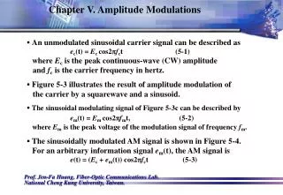
Chapter V. Amplitude Modulations. An unmodulated sinusoidal carrier signal can be described as e c (t) = E c cos2 p f c t (5-1) where E c is the peak continuous-wave (CW) amplitude and f c is the carrier frequency in hertz.

Chapter V. Amplitude Modulations
E N D
Presentation Transcript
Chapter V. Amplitude Modulations • An unmodulated sinusoidal carrier signal can be described as ec(t) = Eccos2pfct (5-1) where Ec is the peak continuous-wave (CW) amplitude and fc is the carrier frequency in hertz. • Figure 5-3 illustrates the result of amplitude modulation of the carrier by a squarewave and a sinusoid. • The sinusoidal modulating signal of Figure 5-3c can be described byem(t) = Emcos2pfmt, (5-2) where Em is the peak voltage of the modulation signal of frequency fm. • The sinusoidally modulated AM signal is shown in Figure 5-4. For an arbitrary information signal em(t), the AM signal is e(t) = (Ec + em(t)) cos2pfct (5-3)
Chapter V. Amplitude Modulations Figure 5-3. Amplitude modulation.
Chapter V. Amplitude Modulations Figure 5-4. (a) Amplitude-modulated signal. (b) Information signal to be transmitted by AM.
Modulation Index • AM modulation index is defined by ma = Em/Ec. Hence, the AM signal can be written for sinusoidal modulation as e(t) = Ec(1+ macos2pfmt) cos2pfct. • A convenient way to measure the AM index is to use an oscilloscope: simply display the AM waveform as in Figure 5-4, and measure the maximum excursion A and the minimum excursion B of the amplitude "envelope" (the information is in the envelope). • The AM index is computed from Figure 5-4 asA = 2(Ec + Em) (5-4a)B = 2(Ec - Em) (5-4b) and, solving for Ec and Em in terms of A and B will then yield (5-4c)
Chapter V. Amplitude Modulations • It should be clear that the peak measurements A/2 and B/2 will yields ma also. The numerical value of mais always in the range of 0 (no modulation) to 1.0 (full modulation) and is usually expressed as a percentage of full modulation. • If more than one sinusoid, such as a musical chord (that is, a triad, 3 tones), modulates the carrier, then we get the resultant AM, index by RMS-averaging the indices that each sine wave would produce. • Thus, in general, ma = (m12 +m22 +m32 +… +mn2)1/2 (5-5)
Chapter V. Amplitude Modulations Figure 5-6. AM represented as the vector sum of sidebands and carrier.
Chapter V. Amplitude Modulations Figure 5-7. (a) ma= 1.0(100% AM). (b) The result of over-modulation that corresponds to the spectrum in (c).
Chapter V. Amplitude Modulations • In Fig. 5-6 the AM signal is shown to be the instantaneous phasor sum of the carrier fc, the lower-side frequency fc–fm, and the upper-side frequency fc+fm. • The phasor addition is shown for six different instants, illustrating how the instantaneous amplitude of the AM signal can be constructed by phasor addition. • Notice how the USB (fc+fm), which is a higher frequency than fc, is steadily gaining on the carrier, while the LSB (fc–fm), a lower frequency, is steadily falling behind.
Chapter V. Amplitude Modulations • The last phasor sketch in Figure 5-6 shows the phasor relationship of sidebands to carrier at the instant corresponding to the minimum amplitude of the AM signal. • You can see that if the amplitude of each sideband is equal to one-half of the carrier amplitude, then the AM envelope goes to zero. • This corresponds to the maximum allowable value of Em; that is, Em =Ecand ma = 1.0 or 100% modulation.
Chapter V. Amplitude Modulations • As illustrated in Figures 5-7b and c, an excessive modulation voltage will result peak clipping and harmonic distortion, which means that additional sidebands are generated. • Not only does over-modulation distortion result in the reception of distorted information, but also the additional sidebands generated usually exceed the maximum bandwidth allowed.
Chapter V. Amplitude Modulations Figure 2-2. The AM signal sisplayed in the frequency domain where fc is the carrier,A is magnitude, the modulating frequency is fixed, and m% is the variable.
Chapter V. Amplitude Modulations Figure 2-3. The signal displayed in the frequency domain where fc is the carrier, A is magnitude, m is constant, and the modulation frequency fm is the variable.
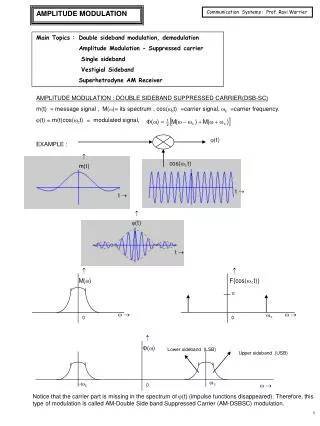
AM SPECTRUM AND BANDWIDTH • Let us analyze the mathematical expression for the AM signal e(t) = (Ec + Emcos2pfmt) cos2pfct = Ec cos2pfct + Emcos2pfmt cos2pfct • The second term of this expression can be expanded by the trigonometric identity cosA.cosB = (1/2)[cos(A-B) + cos(A+B)], so that e(t) = Ec cos2pfct carrier + (Em/2)cos2p(fc-fm)t lower sideband, LSB + (Em/2)cos2p(fc+fm)t upper sideband, USB
AM SPECTRUM AND BANDWIDTH Figure 5-5. Frequency spectrum of the AM signal shown in Figure 5-4.
AM SPECTRUM AND BANDWIDTH Figure 5-11. Amplitude-modulated signal. (a) Generating the AM signal. (b) The AM signal (time domain). (c) The “envelope.” (d) One-sided spectrum of the AM signal (frequency domain).
POWER in an AM SIGNAL • Consider Equation (5-6), if the voltage signal is present on an antenna of effective real impedance R, then the power of each component will be determined from the peak voltages of each sinusoid. • For the carrier, Pc = Ec2/2R, and for each of the two sideband components,
POWER in an AM SIGNAL • Therefore, P1sb = ma2Pc/4 (5-7) where P1sb denotes the power in one sideband only. • The total power in the AM signal will be the sum of these powers: Ptotal = Pc + PLSB + PUSB = Pc + (m2/4)Pc + (m2/4)Pc = Pc(1+ m2/2) = Pt (5-8)
POWER in an AM SIGNAL Relative AM Signal Energy versus Modulation Index %m Energy (Pt/Pc)0 1 10 1.00520 1.02 30 1.045 40 1.08 50 1.125 60 1.18 70 1.245 80 1.32 90 1.405 100 1.5
POWER in an AM SIGNAL • From the tabulation we see that the energy contribution to the carrier is 1/2 that of the carrier itself at 100% modulation. Each of the two sidebands contributes 1/2 of this value or 1/4 of the energy. • As an example, a 100 watt carrier 100% AM by a sine wave, will have an average of 50 watts of sideband power, composed of 25 watts from each sideband.
NONSINUSOIDAL MODULATION SIGNALS • The information signal in modulated systems, as illustrated by Figure 5-8a, is often referred to as the baseband signal, • and the spectrum of Figure 5-8c is the (one-sided) baseband spectrum, where only positive frequencies are shown. • The modulated signal spectrum (one-sided) of Fig. 5-8d consists of the upper and lower sidebands on either side of the carrier. • Figure 5-8d clearly shows that the information bandwidth of the AM signal is 2fm(max).
NONSINUSOIDAL MODULATION SIGNALS Figure 5-8. (a) Information signal (modulation). (b) AM output (time domain). (c) One-sided frequency spectrum of m(t).(d) AM output frequency spectrum (one sided).
NONSINUSOIDAL MODULATION SIGNALS • The mathematically formal method of determining the frequency spectrum of a time-varying signal is to employ the Fourier transform. vAM(t) = Ec.cos2pfct + m(t).cos2pfct (5-9)VAM(f) = (Ec/2)[d(f - fc) + d(f + fc)] + (1/2)[M(f - fc) + M(f + fc)] (5-10)
NONSINUSOIDAL MODULATION SIGNALS • For the two-sided idealized audio frequency spectrum of Figure 5-9a, the plot of Fourier transform of vAM(t), VAM(f), is illustrate in Figure 5-9b. Figure 5-9. (a) Idealized audio time-domain signal and baseband Fourier transform spectrum. (b) Fourier transform spectrum of m(t) amplitude modulated on a (cosine) carrier signal of frequency fc.
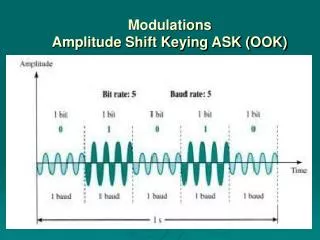
AMPLIIUDE SHIFT KEYING (ASK) or ON/OFF KEYING (OOK) • ASK or OOK consists of a carrier which is turned on, for by a mark and off by a space. The carrier takes on the form of an interrupted carrier, such as in telegraphy, only the data is encoded differently. The signal takes on the form shown in Figure 2-5. • Detection of such a signal may be non-coherent or coherent, with the latter being the better performer, although more difficult to achieve.
AMPLIIUDE SHIFT KEYING (ASK) or ON/OFF KEYING (OOK) Fig. 2-5. The ASK signal in the time domain.
AMPLIIUDE SHIFT KEYING (ASK) or ON/OFF KEYING (OOK) • If the carrier burst is defined as (5-11) then the Fourier transform may be expressed as (5-12) • whered = t/T (5-13) is the duty cycle of the bursts, and T is the pulse repetition period (inverse of the pulse repetition frequency, PRF).
AMPLIIUDE SHIFT KEYING (ASK) or ON/OFF KEYING (OOK) Figure 5-10. 25% duty cycle on-off key (OOK) signal and one-sided frequency spectrum.
AMPLIIUDE SHIFT KEYING (ASK) or ON/OFF KEYING (OOK) Figure 2-6. Non-coherent detection of ASK.
Non-Coherent-Detection of ASK • Non-coherent detector in its simplest form consists of envelope detector followed by decision circuitry, as shown in Fig. 2-6. • The decision threshold grossly affects the error probability (Pe) for mark and space independently, and they are therefore not equally probable. • The “mark” or “carrier on” signal consists of carrier plus noise whereas the “space” or “carrier off” signal is noise alone. It has been shown that Pe(mark) can be made equal to Pe(space) for a given C/N.
Non-Coherent-Detection of ASK • Minimum probability of error results when a thresholds of roughly (pulse-amplitude/2).(1+2Eb/No)1/2(2-8) is used, where Eb is the pulse energyNo is the noise density per reference bandwidth • In general, ASK is a poor performer although it is used in non-critical applications.
Non-Coherent-Detection of ASK • For Eb/No >> 1 and a decision threshold of half the pulse amplitude, the probability of error for space isPe(space) = exp[-(Eb/2No)] (2-9) and for mark Pe(mark) = exp[-(Eb/2No)]/(2pEb/No)1/2 (2-10) • From this, it is seen that the majority of errors are spaces converted to marks.
Coherent Detection of ASK • Coherent detection requires a product detector with a reference signal which is phase coherent with the incoming signal carrier (see Figure 2-7). • The product detector is followed by an integrator and a decision circuit timed to function at the end of bit time t. Fig. 2-7. Coherent detection of ASK using synchronous detection.
Coherent Detection of ASK • An equivalent performer is the matched-filter detector shown in Figure 2-8. • Here, the output of the matched filter is the convolution of the pulse and the impulse response of the matched filter. • The resulting output is ideally diamond shaped and of duration 2t, with maximum signal energy at a time of A2/2, where A is the signal amplitude and t is the pulse duration. • To complete the system, the decision circuitry is timed to function at time t for optimum performance.
Coherent Detection of ASK Fig. 2-8. Matched filter detection of ASK signals.
Coherent Detection of ASK • The probability of error for coherent ASK signaling is: (2-11)
AM DEMODULATION Figure 5-13. Peak amplitude detector. • The diode shown in Figure 5-13 conducts whenever vin exceeds the diode cut-in voltage of about 0.2V for germanium. Hence, with no capacitor, the detector output is just the positive peaks of the input AM signal. • The value of vo will rise and fall at the same rate as the information -- 5 kHz in this case. All that is required is some filtering to smooth out the recovered information.
AM DEMODULATION • If a capacitor is added to the circuit, as shown in Fig. 5-14, not only is filtering provided but also the average value of the demodulated signal is increased. • The capacitor charged up to the positive peak value of the carrier pulse while the diode is conducting. • The capacitor is allowed to discharge just slowly enough through the resistor that the very next carrier peak will exceed vo, thereby allowing the diode to conduct and charge the capacitor up to the new peak value. • The result is that the output voltage will follow the input AM peaks with a loss of only the voltage dropped across the diode.
AM DEMODULATION Figure 5-14. AM demodulation.
Diagonal Clipping Distortion • The values of R and C at the output of the AM detector must be chosen to optimize the demodulation process. As illustrated in Figure 5-15, if the capacitor is too large, it will not be able to discharge fast enough for vo to follow the fast variations of the AM envelope. • The result will be that much of the information will be lost during the discharge time. This effect is called diagonal clipping because of the diagonal appearance of the discharge curve. • The distortion that results, however, is not just poor sound quality (fidelity) as for peak clipping; it can also result in a considerable loss of information.
Diagonal Clipping Distortion Figure 5-15. Diagonal clipping.
Diagonal Clipping Distortion • The optimum time constant is determined by analyzing the diagonal clipping problem. Compare the RC discharge rate required for the low modulation index illustrated in Figure 5-16a with that required for the same modulating signal but higher index seen in b. • Clearly, the modulation index is an important parameter, and the appropriate RC time constant depends not only on the highest modulating frequency fm(max), but also on the depth or percentage of modulation ma. In fact, the maximum value of C is determined from Equation (5-16). (5-16)
Diagonal Clipping Distortion Figure 5-16. A higher-index AM requires a shorter RC time constant.
Diagonal Clipping Distortion Figure 5-17. Complete AM detector and volume (loudness) control.
Diagonal Clipping Distortion • In 5-17, the demodulated information signal is ac coupled by capacitor Cc to the audio amplifiers. Coupling capacitor Cc is made large enough to pass the lowest audio frequencies while blocking the dc bias of the audio amplifier and the average (dc) value of vo. • The audio amplifier input impedance ZA should be much greater than the output impedance of the detector R to avoid peak clipping distortion that occurs when the peak ac current required by ZA is greater than the average current available.
SUPERHETERODYNE RECEIVERS • The standard AM broadcast band in North America extends from 535 to 1605 kHz, with transmitted carrier frequencies every 10 kHz from 540 to 1600 kHz (20Hz tolerance). • The 10 kHz of separation AM stations allows for a maximum modulation frequency of 5 kHz. Figure 5-19. Superheterodyne receiver.
SUPERHETERODYNE RECEIVERS • Indeed, many use a second down conversion and second IF amplifier system following the first IF. Such a super- heterodyne receiver is called a double-conversion receiver. • The LO frequency is almost always higher than the RF carrier frequency, a characteristic referred to as high-side injection to the mixer. • For example, to receive the AM station whose RF carrier is fRF = 560kHz, the LO must be tuned to fLO = fRF + fIF = 560 kHz + 455 kHz = 1015 kHz
Choice of IF Frequency and Image Response • Receiver selectivity, tuning in one station while rejecting interference from all others, is determined by filtering at the receiver RF input and in the IF. Figure 5-20. IF filter at mixer output.
Choice of IF Frequency and Image Response • Adjacent channels are rejected primarily by IF filtering. Filter out adjacent channel transmissions right at the RF input are difficult. • The first considerationis that the RF input circuit may be required to tune over a relatively wide frequency range. Maintaining a high Q and constant bandwidth in such a circuit is very difficult. • The second consideration is that multipole networks are employed. Tuning a multiple filter from station to station over even a moderate tuning range is not practical.
Choice of IF Frequency and Image Response • The image frequency is that frequency which is exactly one IF frequency above the LO when high-side injection is used. That is,fimage = fLO + fIF = fRF + 2fIF. • Image response rejection is achieved by filtering before the mixer. • An AM receiver (IF = 455kHz) is tuned to receive a station whose carrier frequency is fRF = 1MHz. The LO is fLO = 1.455 MHz and the interfering signal is at 1.910 MHz. • Consequently the difference frequency is 1.910 MHz – 1.455 MHz = 455 kHz, exactly our IF center frequency!
RECEIVER GAIN and SENSITIVITY • Suppose a 90% AM signal is received, the receiver must amplify this until it is large enough to cause the diode to conduct. Indeed to prevent negative peak distortion at the detector, the minimum positive peak Vmin must cause conduction. • A conservative figure for Vmin when using a germanium detector diode is about 0.2V, including junction potential and I2R losses in the diode and detector circuitry. • Referring to Figure 5-4, Vc is the average value between A • and B; that is Vc = (A+B)/2. Notice also that B = Vmin, so we • solve for B in terms of A in m = (A–B)/(A+B) which gives A = [(1+m)/(1-m)]B (5-20)