Download
1 / 31
310 likes | 334 Views
Cost-Revenue Analysis Break-Even Points. The Cost Function , C(q), gives the total cost of producing a quantity q of some good. What sort of function do you expect C(q) to be?

E N D
Cost-Revenue AnalysisBreak-Even Points The Cost Function, C(q), gives the total cost of producing a quantity q of some good. What sort of function do you expect C(q) to be? The more goods that are made, the higher the total cost, so C(q) is an increasing function. Costs of production can be separated into two parts: the fixed costs, which are incurred even if nothing is produced, and the variable cost, which depends on how many units are produced.
Cost-Revenue AnalysisBreak-Even Points Let’s consider a company that makes radios. The factory and machinery needed to begin production are fixed costs, which are incurred even if no radios are made. The costs of labor and raw materials are variable costs since these quantities depend on how many radios are made. The fixed costs for this company are $24,000 and the variable costs are $7 per radio. Then, Total cost for the company = Fixed costs + Variable costs = 24,000 + 7 • Number of radios, So, if q is the number of radios produced, C(q) = 24,000 + 7q. This is the equation of a line with slope 7 and vertical intercept of 24,000.
Cost-Revenue AnalysisBreak-Even Points Example 1: Graph the cost function C(q) = 24,000 + 7q. Label the fixed costs and variable cost per unit. Solution: The graph of the cost function is the line in the figure below. The fixed costs are represented by the vertical intercept of 24,000. The variable cost per unit is represented by the slope of 7, which is the change in cost corresponding to unit change in production.
Cost-Revenue AnalysisBreak-Even Points Notes: If C(q) is a linear cost function, Fixed costs are represented by the vertical intercept. Variable costs per unit are represented by the slope.
Cost-Revenue AnalysisBreak-Even Points Example 2: In each case, draw a graph of a linear cost function satisfying the given conditions: Fixed costs are larger but variable cost per unit is small. There are no fixed costs but a large variable cost per unit length.
Cost-Revenue AnalysisBreak-Even Points Example 2: In each case, draw a graph of a linear cost function satisfying the given conditions: The graph is a line with a large vertical intercept and a small slope.
Cost-Revenue AnalysisBreak-Even Points Example 2:In each case, draw a graph of a linear cost function satisfying the given conditions: (b) The graph is a line with a vertical intercept of zero (so the line goes through the origin) and a large positive slope.
Cost-Revenue AnalysisBreak-Even Points The Revenue Function, R(q), gives the total revenue received by a firm from selling a quantity, q, of some good. If the good sells for a price of p per unit, and the quantity sold is q, then Revenue = Price • Quantity, so R = pq. If the price does not depend on the quantity sold, so p is a constant, the graph of revenue as a function of q is a line through the origin, with slope equal to the price p.
Cost-Revenue AnalysisBreak-Even Points Example 3: If radios sell for $15 each, sketch the manufacturer’s revenue function. Show the price of a radio on the graph. Solution: Since R(q) = pq = 15q, the revenue graph is a line through the origin with a slope of 15.
Cost-Revenue AnalysisBreak-Even Points Example 4: Sketch graphs of the cost function C(q) = 24,000 + 7q and revenue function R(q) = 15q on the same axes. For what values of q does the company make money? Explain your answer graphically. Solution: The company makes money whenever revenues are greater than costs, so we want to find the values of q for which the graph of R(q) lies above the graph of C(q). We find the point at which the graphs of R(q) and C(q) cross:
Cost-Revenue AnalysisBreak-Even Points Example 4: Sketch graphs of the cost function C(q) = 24,000 + 7q and revenue function R(q) = 15q on the same axes. For what values of q does the company make money? Explain your answer graphically. Revenue = Cost 15q = 24,000 + 7q 8q = 24,000 q = 3000 Thus, the company makes a profit if it produces and sells more than 3000 radios. The company loses money if it produces and sells fewer than 3000 radios.
Cost-Revenue AnalysisBreak-Even Points Example 4: Sketch graphs of the cost function C(q) = 24,000 + 7q and revenue function R(q) = 15q on the same axes. For what values of q does the company make money? Explain your answer graphically.
Cost-Revenue AnalysisBreak-Even Points The Profit Function: Decisions are often made by considering the profit, usually written as π to distinguish it from the price, p. We have Profit = Revenue - Cost so π = R - C. The break-even point for a company is the point where the profit is zero and revenue equals cost. A break-even point can refer either to a quantity q at which revenue equals cost, or to a point on a graph.
Cost-Revenue AnalysisBreak-Even Points Example 5: Find a formula for the profit function of the radio manufacturer. Graph it, marking the break-even point. Solution: Since R(q) = 15q and C(q) = 24,000 + 7q, we have, π(q) = 15q - (24,000 + 7q) = -24,000 + 8q Notice that the negative of the fixed costs is the vertical intercept and the break-even point is the horizontal intercept.
Cost-Revenue AnalysisBreak-Even Points Example 5: Find a formula for the profit function of the radio manufacturer. Graph it, marking the break-even point.
Cost-Revenue AnalysisBreak-Even Points The Marginal Cost, Marginal Revenue, and Marginal Profit In economics and business, the terms marginal cost, marginal revenue, and marginal profit are used for the rate of change of cost, revenue, and profit, respectively. The term marginal is used to highlight the rate of change as an indicator of how the cost, revenue, or profit changes in response to one unit (that is, marginal) change in quantity. For example, for the cost, revenue, and profit functions of the radio manufacturer, the marginal cost is 7 dollars/item (the additional cost of producing one more item is $7), the marginal revenue is 15 dollars/item (the additional revenue from selling one more item is $15), and the marginal profit is 8 dollars/item (the additional profit from selling one more item is $8).
Cost-Revenue AnalysisBreak-Even Points The Depreciation Function Suppose that the radio manufacturer has a machine that costs $20,000. The managers of the company plan to keep the machine for ten years and then sell it for $3000. We say the value of their machine depreciates from $20,000 today to a resale value of $3000 in ten years. The depreciation formula gives the value, V(t), of the machine as a function of the number of years, t, since the machine was purchased. We assume that the value of the machine depreciates linearly. The value of the machine when it is new (t = 0) is $20,000, so V(0) = 20,000. The resale value at time t = 10 is $3000, so V(10) = 3000. We have
Cost-Revenue AnalysisBreak-Even Points The Depreciation Function This slope tells us that the value of the machine is decreasing at a rate of $1700 per year. Since V(0) = 20,000, the vertical intercept is 20,000, so V(t) = 20,000 - 1700t
Cost-Revenue AnalysisBreak-Even Points Supply and Demand Curves: The quantity, q, of an item that is manufactured and sold, depends on its price, p. We usually assume that as the price increases, manufacturers are willing to supply more of the product, whereas the quantity demanded by consumers falls. Since manufacturers and consumers react differently to changes in price, there are two curves relating p and q.
Cost-Revenue AnalysisBreak-Even Points The supply curve, for a given item, relates the quantity, q, of the item that manufacturers are willing to make per unit time to the price, p, for which the item can be sold. The demand curve relates the quantity, q, of an item demanded by consumers per unit time to the price, p, of the item.
Cost-Revenue AnalysisBreak-Even Points Economists often think of the quantities supplied and demanded as functions of price. However, for historical reasons, the economists put price (the independent variable) on the vertical axis and quantity (the dependent variable) on the horizontal axis. (The reason for this state of affairs is that economists originally took price to be the dependent variable and put it on the vertical axis. Later, when the point of view changed, the axes did not.) Thus, typically supply and demand curves look like these shown on the next slide….
Cost-Revenue AnalysisBreak-Even Points Example 6: What is the economic meaning of the prices p0 and p1 and the quantity q1 in the graph on the previous slide? Solution: The vertical axis corresponds to a quantity of zero. Since the price p0 is the vertical intercept on the supply curve, p0 is the price at which the quantity supplied is zero. In other words, unless the price is above p0, the suppliers will not produce anything. The price p1 is the vertical intercept on the demand curve, so it corresponds to the price at which the quantity demanded is zero. In other words, unless the price is below p1, consumers won’t buy any of the product. The horizontal axis corresponds to a price of zero, so the quantity q1 on the demand curve is the quantity that would be demanded if the price were zero - or the quantity that could be given away if the item were free.
Cost-Revenue AnalysisBreak-Even Points Equilibrium Price and Quantity If we plot the supply and demand curves on the same axes, the graphs cross at the equilibrium point. The values p and q at this point are called the equilibrium price and equilibrium quantity, respectively. It is assumed that the market naturally settles to this equilibrium point.
Cost-Revenue AnalysisBreak-Even Points Example 7: Find the equilibrium price and quantity if Quantity supplied = S(p) = 3p - 50 and Quantity demanded = D(p) = 100 - 2p. Solution: To find the equilibrium price and quantity, we find the point at which Supply = Demand 3p - 50 = 100 - 2p 5p = 150 p = 30
Cost-Revenue AnalysisBreak-Even Points The equilibrium price is $30. To find the equilibrium quantity, we use either the demand curve or the supply curve. At a price of $30, the quantity produced is 100 - 2(30) = 100 - 60 = 40 items. The equilibrium quantity is 40 items. In the figure below, the demand and supply curves intersect at p = 30 and q = 40.
Cost-Revenue AnalysisBreak-Even Points Question: What effect do taxes have on the equilibrium price and quantity for this product? And who (the producer or consumer) ends up paying for the tax? We distinguish between two types of taxes. A specific tax is a fixed amount per unit of a product sold regardless of the selling price. This is the case with such items as gasoline, alcohol, and cigarettes. A specific tax is usually imposed on the producer. A sales tax is a fixed percentage of the selling price. Many cities and states collect sales tax on a wide variety of items. A sales tax is usually imposed on the consumer. We consider a specific tax on the next slide.
Cost-Revenue AnalysisBreak-Even Points Suppose a specific tax of $5 per unit is imposed upon suppliers. This means that a selling price of p dollars does not bring forth the same quantity supplied as before, since suppliers only receive p - 5 dollars. The amount supplied corresponds to p - 5, while the amount demanded still corresponds to p, the price the consumers pay. We have Quantity demanded = D(p) = 100 - 2p Quantity supplied = S(p - 5) = 3(p - 5) - 50 = 3p - 15 - 50 = 3p - 65
Cost-Revenue AnalysisBreak-Even Points What are the equilibrium price and quantity in this situation? At the equilibrium price, we have Demand = Supply 100 - 2p = 3p - 65 165 = 5p p = 33 The equilibrium price is now $33. However, before the equilibrium price was $30, so the equilibrium price increased by $3 as a result of the tax. Notice that this is less than the amount of the tax.
Cost-Revenue AnalysisBreak-Even Points The consumer ends up paying $3 more than if the tax did not exist. However, the government receives $5 per item. Thus the producer pays the other $2 of the tax, retaining $28 of the price paid per item. Thus, although the tax was imposed on the producer, some of the tax is passed on to the consumer in terms of higher prices. The actual cost of the tax is split between the consumer and the producer. The equilibrium quantity is now 34 units, since the quantity demanded is D(33) = 34. Not surprisingly, the tax has reduced the number of items sold. See figure on next slide…