CE 400 Honors Seminar Molecular Simulation

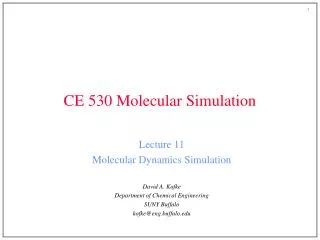
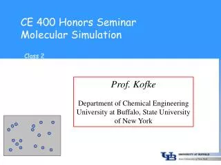
CE 400 Honors SeminarMolecular Simulation Class 2 Prof. Kofke Department of Chemical Engineering University at Buffalo, State University of New York

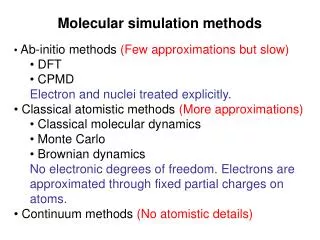
Review: What is Molecular Simulation? • Molecular simulation is a computational “experiment” conducted on a molecular model. • Many configurations are generated, and averages taken to yield the “measurements.” One of two methods is used: • Molecular dynamics Monte Carlo • Integration of equations of motion Ensemble average • Deterministic Stochastic • Retains time element No element of time • Molecular simulation has the character of both theory and experiment • Applicable to molecules ranging in complexity from rare gases to polymers to electrolytes to metals 10 to 100,000 or more atoms are simulated (typically 500 - 1000)

Etomica • GUI-based development environment • Simulation is constructed by piecing together elements • No programming required • Result can be exported to run stand-alone as applet or application • Application Programming Interface (API) • Library of components used to assemble a simulation • Can be used independent of development environment • Invoked in code programmed using Emacs or Wordpad (for example) • Written in Java • Widely used and platform independent • Features of a modern programming language • Object-oriented • Java Reference: “Thinking in Java” by Bruce Eckel • Available free online at www.bruceeckel.com

What is an Object? • A fancy variable • stores data • can perform operations using the data • Every object has a type, or “class” • analogous to real, integer, etc. • Fortran: real x, y, z • Java: Atom a1, a2; • you define types (classes) as needed to solve your problems public class Atom { double mass; Vector r, p; } • types differ in the data they hold and the actions they perform • every object is an “instance of a class” a1 = new Atom();

Makeup of an Object • Fields (data) • primitive types (integer, float, double, boolean, etc.) • handles to other objects • complex objects are composed from simpler objects (composition) • Methods (actions) • “subroutines and functions” • may take arguments and return values • have complete access to all fields of object • Inheritance • can define subclasses which inherit features of parent class • same interface, but different implementations • subclasses can be used anywhere parent class is expected • mechanism to change behavior of simulation

Structure of a Molecular Simulation Initialization Reset block sums “cycle” or “sweep” New configuration “block” moves per cycle Move each atom once (on average) Add to block sum 100’s or 1000’s of cycles Independent “measurement” cycles per block Compute block average blocks per simulation Compute final results

Simulation Element: Integrator • Advances molecule positions according to some rule • Here’s the core method in parent Integrator class public void run() { stepCount = 0; int iieCount = interval+1; while(stepCount < maxSteps) { while(pauseRequested) doWait(); if(resetRequested) {doReset(); resetRequested = false;} if(haltRequested) break; doStep();//abstract method in Integrator. subclasses implement algorithms (MD/MC) if(--iieCount == 0) { //count down to determine when a cycle is completed fireIntervalEvent(intervalEvent); //notify listeners of completion of cycle iieCount = interval; } if(doSleep) { //slow down simulation so display can keep up try { Thread.sleep(sleepPeriod); } catch (InterruptedException e) { } } stepCount++; } //end of while loop fireIntervalEvent(new IntervalEvent(this, IntervalEvent.DONE)); } //end of run method

Integration Algorithms • Equations of motion in cartesian coordinates • Desirable features of an integrator • minimal need to compute forces (a very expensive calculation) • good stability for large time steps • good accuracy • conserves energy and momentum • Soft- and hard-potential integrators work differently 2-dimensional space (for example) pairwise additive forces F

Verlet Algorithm 1. Equations • Very simple, very good, very popular algorithm • Consider expansion of coordinate forward and backward in time

Verlet Algorithm 1. Equations • Very simple, very good, very popular algorithm • Consider expansion of coordinate forward and backward in time • Add these together

Verlet Algorithm 1. Equations • Very simple, very good, very popular algorithm • Consider expansion of coordinate forward and backward in time • Add these together • Rearrange • update without ever consulting velocities!

Verlet Algorithm 2. Flow diagram One MD Cycle Configuration r(t) Previous configuration r(t-dt) Entire Simulation Initialization One force evaluation per time step Compute forces F(t) on all atoms using r(t) Reset block sums New configuration 1 move per cycle Advance all positions according to r(t+dt) = 2r(t)-r(t-dt)+F(t)/m dt2 Add to block sum cycles per block Compute block average blocks per simulation Add to block sum Compute final results No End of block? Yes Block averages

Verlet Algorithm 3. Java Code run() method in Integrator public void run() { stepCount = 0; int iieCount = interval+1; while(stepCount < maxSteps) { while(pauseRequested) doWait(); if(resetRequested) {doReset();} if(haltRequested) break; doStep(); if(--iieCount == 0) { fireIntervalEvent(); iieCount = interval; } if(doSleep) { } stepCount++; } //end of while loop fireIntervalEvent(); } //end of run method • Time for a demonstration… public class IntegratorVerlet extends Integrator //Performs one timestep increment in the Verlet algorithm public void doStep() { atomIterator.reset(); while(atomIterator.hasNext()) { //zero forces on all atoms ((Agent)atomIterator.next().ia).force.E(0.0); } pairIterator.allPairs(forceSum); //sum forces on all pairs double t2 = tStep*tStep; atomIterator.reset(); while(atomIterator.hasNext()) { //loop over all atoms, moving according to Verlet Atom a = atomIterator.next(); Agent agent = (Agent)a.ia; Space.Vector r = a.position(); //current position of the atom temp.E(r); //save it r.TE(2.0); //2*r r.ME(agent.rLast); //2*r-rLast agent.force.TE(a.rm()*t2); // f/m dt^2 r.PE(agent.force); //2*r - rLast + f/m dt^2 agent.rLast.E(temp); //rLast gets present r } return; }

Verlet Algorithm 3. Java Code • Time for a demonstration… public class IntegratorVerlet extends Integrator //Performs one timestep increment in the Verlet algorithm public void doStep() { atomIterator.reset(); while(atomIterator.hasNext()) { //zero forces on all atoms ((Agent)atomIterator.next().ia).force.E(0.0); } pairIterator.allPairs(forceSum); //sum forces on all pairs double t2 = tStep*tStep; atomIterator.reset(); while(atomIterator.hasNext()) { //loop over all atoms, moving according to Verlet Atom a = atomIterator.next(); Agent agent = (Agent)a.ia; Space.Vector r = a.position(); //current position of the atom temp.E(r); //save it r.TE(2.0); //2*r r.ME(agent.rLast); //2*r-rLast agent.force.TE(a.rm()*t2); // f/m dt^2 r.PE(agent.force); //2*r - rLast + f/m dt^2 agent.rLast.E(temp); //rLast gets present r } return; }

Monte Carlo Simulation 1. • Gives properties via ensemble averaging • No time integration • Cannot measure dynamical properties • Employs stochastic methods to generate a (large) sample of members of an ensemble • “random numbers” guide the selection of new samples • Permits great flexibility • members of ensemble can be generated according to any convenient probability distribution… • …and probability distribution can be sampled many ways • strategies developed to optimize quality of results • ergodicity — better sampling of all relevant regions of configuration space • variance minimization — better precision of results • MC “simulation” is the evaluation of statistical-mechanics integrals

Monte Carlo Simulation 2. State k • Almost always involves a Markov process • move to a new configuration from an existing one according to a well-defined transition probability • Simulation procedure • generate a new “trial” configuration by making a perturbation to the present configuration • accept the new configuration based on the ratio of the probabilities for the new and old configurations, according to the Metropolis algorithm • if the trial is rejected, the present configuration is taken as the next one in the Markov chain • repeat this many times, accumulating sums for averages State k+1

Trial Moves • A great variety of trial moves can be made • Basic selection of trial moves is dictated by choice of ensemble • almost all MC is performed at constant T • no need to ensure trial holds energy fixed • must ensure relevant elements of ensemble are sampled • all ensembles have molecule displacement, rotation; atom displacement • isobaric ensembles have trials that change the volume • grand-canonical ensembles have trials that insert/delete a molecule • Significant increase in efficiency of algorithm can be achieved by the introduction of clever trial moves • reptation, crankshaft moves for polymers • multi-molecule movements of associating molecules • many more

General Form of MC Algorithm Entire Simulation Initialization Reset block sums “cycle” or “sweep” New configuration “block” moves per cycle Add to block sum cycles per block Compute block average blocks per simulation Compute final results Monte Carlo Move New configuration Select type of trial move each type of move has fixed probability of being selected Move each atom once (on average) 100’s or 1000’s of cycles Independent “measurement” Perform selected trial move Decide to accept trial configuration, or keep original

Monte Carlo Integrator run() method in Integrator public void run() { stepCount = 0; int iieCount = interval+1; while(stepCount < maxSteps) { while(pauseRequested) doWait(); if(resetRequested) {doReset();} if(haltRequested) break; doStep(); if(--iieCount == 0) { fireIntervalEvent(); iieCount = interval; } if(doSleep) { } stepCount++; } //end of while loop fireIntervalEvent(); } //end of run method • Here’s the core method in IntegratorMC class • All the work is done by the MCMove class public class IntegratorMC extends Integrator public void doStep() { int i = (int)(rand.nextDouble()*frequencyTotal); //select trial MCMove trialMove = firstMove; while((i-=trialMove.getFrequency()) >= 0) { trialMove = trialMove.nextMove(); } trialMove.doTrial(); //perform trial move and decide acceptance } public class MCMove public void doTrial() { nTrials++; thisTrial(); if(relaxation && nTrials > adjustInterval*frequency) {adjustStepSize();} }

Monte Carlo Integrator • Here’s the core method in IntegratorMC class • All the work is done by the MCMove class public class IntegratorMC extends Integrator public void doStep() { int i = (int)(rand.nextDouble()*frequencyTotal); //select trial MCMove trialMove = firstMove; while((i-=trialMove.getFrequency()) >= 0) { trialMove = trialMove.nextMove(); } trialMove.doTrial(); //perform trial move and decide acceptance } public class MCMove public void doTrial() { nTrials++; thisTrial(); if(relaxation && nTrials > adjustInterval*frequency) {adjustStepSize();} }

Displacement Trial • Gives new configuration of same volume and number of molecules • Basic trial: • displace a randomly selected atom to a point chosen with uniform probability inside a cubic volume of edge 2d centered on the current position of the atom Move atom to point chosen uniformly in region

Displacement Trial • Gives new configuration of same volume and number of molecules • Basic trial: • displace a randomly selected atom to a point chosen with uniform probability inside a cubic volume of edge 2d centered on the current position of the atom Consider acceptance of new configuration ?

Displacement Trial • Gives new configuration of same volume and number of molecules • Basic trial: • displace a randomly selected atom to a point chosen with uniform probability inside a cubic volume of edge 2d centered on the current position of the atom • Limiting probability distribution • canonical ensemble Examine underlying transition probabilities to formulate acceptance criterion ?

Analysis of Trial Probabilities • Detailed specification of trial moves and probabilities Forward-step trial probability Reverse-step trial probability v = (2d)d c is formulated to satisfy detailed balance

Analysis of Detailed Balance Forward-step trial probability Reverse-step trial probability pi pij pj pji Detailed balance = Limiting distribution

Analysis of Detailed Balance Forward-step trial probability Reverse-step trial probability pi pij pj pji Detailed balance = Acceptance probability

Examination of Java Code public class MCMoveAtom extends MCMove public void thisTrial(Phase phase) { double uOld, uNew; if(phase.atomCount==0) {return;} //no atoms to move Atom a = phase.randomAtom(); uOld = phase.potentialEnergy.currentValue(a); //calculate its contribution to the energy a.displaceWithin(stepSize); //move it within a local volume uNew = phase.potentialEnergy.currentValue(a); //calculate its new contribution to energy if(uNew < uOld) { //accept if energy decreased nAccept++; return; } if(uNew >= Double.MAX_VALUE || //reject if energy is huge or doesn’t pass test Math.exp(-(uNew-uOld)/parentIntegrator.temperature) < rand.nextDouble()) { a.replace(); //...put it back in its original position return; } nAccept++; //if reached here, move is accepted } • Time for a demonstration…

Summary: Integrator Class Structure Integrator abstract doStep() IntegratorVerlet doStep(){…} IntegratorGear4 doStep(){…} IntegratorMC doStep(){ selectMove move.doTrial } etc. MCMoveAtom doTrial(){…} MCMoveRotate doTrial(){…} MCMoveInsertDelete doTrial(){…} etc.

Simulation Element: Meter • Measures some property of interest • Keeps average • Coordinates block averaging and error analysis • Can keep history and histograms Entire Simulation Initialization Reset block sums New configuration 1 move per cycle Add to block sum cycles per block Compute block average blocks per simulation Compute final results

Integrator Events • Integrator notifies listeners when it has made some progress • Remember core method in Integrator class public void run() { stepCount = 0; int iieCount = interval+1; while(stepCount < maxSteps) { while(pauseRequested) doWait(); if(resetRequested) {doReset(); resetRequested = false;} if(haltRequested) break; doStep(); //abstract method in Integrator. subclasses implement algorithms (MD/MC) if(--iieCount == 0) {//count down to determine when a cycle is completed fireIntervalEvent(intervalEvent);//notify listeners of completion of cycle iieCount = interval; } if(doSleep) { //slow down simulation so display can keep up try { Thread.sleep(sleepPeriod); } catch (InterruptedException e) { } } stepCount++; } //end of while loop fireIntervalEvent(new IntervalEvent(this, IntervalEvent.DONE)); } //end of run method

All Meters are Integrator Listeners • On receiving event, meter takes action to measure its property • Each meter implements a different currentValue method public abstract class MeterAbstract public void intervalAction(Integrator.IntervalEvent evt) { if(!active) return; if(evt.type() != Integrator.IntervalEvent.INTERVAL) return; //don't act on start, done, etc if(--iieCount == 0) { iieCount = updateInterval; accumulator.add(currentValue()); } } public abstract double currentValue();

Accumulator Does the Bookkeeping public class Accumulator public void add(double value) { mostRecent = value; if(Double.isNaN(value)) return; blockSum += value; if(--blockCountDown == 0) { //count down to zero to determine completion of block blockSum /= blockSize; //compute block average sum += blockSum; sumSquare += blockSum*blockSum; count++; if(count > 1) { double avg = sum/(double)count; error = Math.sqrt((sumSquare/(double)count - avg*avg)/(double)(count-1)); } //reset blocks mostRecentBlock = blockSum; blockCountDown = blockSize; blockSum = 0.0; } if(histogramming) histogram.addValue(value); if(historying) history.addValue(value); }

Some Meter Implementations public class MeterDensity public double currentValue() { return phase.moleculeCount / phase.volume(); } public class MeterKineticEnergy public double currentValue() { double ke = 0.0; atomIterator.reset(); while(atomIterator.hasNext()) { ke += atomIterator.next().kineticEnergy(); } return ke; } public class MeterPressureHard public double currentValue() { double t = integrator.elapsedTime(); if(t > t0) { double flux = -virialSum/((t-t0)*D*phase.atomCount()); value = integrator.temperature() + flux; t0 = t; virialSum = 0.0; } return value; } • Time for a demonstration…

Simulation Elements: Displays and Devices • Displays: Output of information • Integrator listener…update when informed of integrator’s progress • Plot: graphical display • Table: tabular display • Box: single value in a box • Log: write results to a log file • Phase: animation of atom positions • Devices: Input of data and manipulation of simulation • Slider: connects to a property • Table: property-sheet like adjustment of values • Temperature chooser: comboBox selection of temperatures • Most Displays/Devices oriented toward interactive use • Let’s demonstrate…

Simulation Elements: Species and Potentials • Species: Data structure • Control of number of molecules, atoms per molecule • Atom positions, velocities, masses, shapes • Examples • Spheres, walls • Specific elements and compounds (H2O) appear as special cases • Potentials: How atoms interact • Soft potentials • Energy, force, virial • Hard potentials • Energy, collision time, collision dynamics • Examples • Lennard-Jones, hard spheres, square well, etc. • Let’s demonstrate…

Simulation Element: Phase • Phase collects all the molecules that are interacting • Holds boundary conditions • Let’s see… • Normally have one phase per simulation… • …but some simulation techniques work with several phases simulataneously • Methods for evaluation of phase equilibria • Gibbs ensemble • Gibbs-Duhem integration • Sampling-enhancement methods • Parallel tempering • Let’s build a Gibbs-ensemble simulation… • But first: what is the Gibbs ensemble?

Phase Equilibria: Direct Methods • Heating or cooling of one phase • severe hysteresis • e.g., LJ: Tf = 0.48, Tm = 0.84 (thermodynamic value: 0.687) • useful only for bounding transition region • not quantitatively accurate • Multiphase system • Interface dominates behavior • Neither bulk phase is well represented

Gibbs ensemble Two simulation volumes • Method of choice for fluid-phase equilibria A.Z. Panagiotopoulos, Mol. Phys.61, 813 (1987) Particle exchange equilibrates fugacity Volume exchange equilibrates pressure

Simulation Element: Space • “Behind the scenes” simulation element • Provides data structures for positions, velocities, rotations, tensors and phase boundaries • Permits arbitrary specification of spatial dimension • Must select when beginning to construct simulation • For example… public class Space2D.Vector public double x, y; public void E(Vector u) {x = u.x; y = u.y;} //set one vector equal to another public void PE(Vector u) {x += u.x; y += u.y;} //add one vector to another public void TE(double a) {x *= a; y *= a;} //multiply a vector by a scalar public void TE(Vector u) {x *= u.x; y *= u.y;} //multiply vectors term by term public double squared() {return x*x + y*y;} //square of vector magnitude public double dot(Vector u) {return x*u.x + y*u.y;} //dot product of vector with another etc.

Simulation Element: Controller Entire Simulation Entire Simulation Entire Simulation Initialization Initialization Initialization Reset block sums Reset block sums Reset block sums New configuration New configuration New configuration 1 move per cycle 1 move per cycle 1 move per cycle Add to block sum Add to block sum Add to block sum cycles per block cycles per block cycles per block Compute block average Compute block average Compute block average blocks per simulation blocks per simulation blocks per simulation Compute final results Compute final results Compute final results • Controls when simulations start and what happens when they finish. For example… • On and off with a button • Equilibration, production, finish • Perform series of simulations • Thermodynamic integration, Gibbs-Duhem integration • Set state conditions and turn integrator(s) on and off

Saving/Exporting Simulations with Etomica • Serialization (Java technology for saving objects) • Saves simulation in its present state (even after running) • Can read back into Etomica and continue • Can import as an applet to a web page (almost) • Write out as Java source • Saves changes made by Etomica editor, but not changes from running simulation • Save as application or (to be implemented) applet • Need to compile and (if applet) write html page separately • Some further development needed • Let’s see…

Etomica is Extensible • New components easily added • Selection of simulation elements is constructed on-the-fly, by examining files in class path • Introspective • Editable properties of components discovered automatically • Classes should conform to (extended) Javabeans specification public class SpeciesDisks public double getMass() {return mass;} public void setMass(double mass) {mass = m;} public Dimension getMassDimension() {return Dimension.MASS;} public double getDiameter() {return diameter;} public void setDiameter(double d) {diameter = d;} public Dimension getDiameterDimension() {return Dimension.LENGTH;}

Adding New Simulation Elements • Download the following files • www.cheme.buffalo.edu/courses/ce400/DeviceNSelector.class • www.cheme.buffalo.edu/courses/ce400/DeviceNSelector$1.class • www.cheme.buffalo.edu/courses/ce400/DeviceNSelector$2.class • www.cheme.buffalo.edu/courses/ce400/DeviceNSelector$3.class • Save each in your Etomica class directory • Can’t do this in Furnas 1019 lab! • Start up Etomica • Prepare a new simulation, adding this device first

Summary: Etomica Class Structure Simulation Organization and reference Space 1-D, 2-D, 3-D, lattice, etc. Vector, Tensor, Boundary Phase Container of molecules Species Molecule data structure Potential Molecule interactions Controller Protocol for simulation Integrator Generation of configurations Meter Property measurement Modulator Changing of parameters Display Presentation of data Device Interaction with simulation Support Units, Iterators, Atom types, Actions, Color schemes, Constants, Defaults, Configurations

Etomica Web Site • www.ccr.buffalo.edu/etomica • Can download Etomica to your own computer • Some documentation • Source files • Links to other applets

Assignment #0 • Send me an email • kofke@eng.buffalo.edu

Assignment #1 • Construct a simple molecular simulation in Etomica • Hard-sphere or square-well molecular dynamics; vary temperature and density, measure pressure • Lennard-Jones Monte Carlo, vary temperature and pressure, measure density • Export it as an applet and make it accessible on a web site • Perform “experiments” using your simulation • Vary one or two properties and measure another • Make a plot of your data • Comment on your findings • Put everything on a web site • Working applet • Figures • Analysis/commentary • Complete in one week (October 2) • Work in your group

Deploying an Applet 1. • Construct simulation in Etomica • Use “File/Write Java source” to create simulation source file • For example, MySimulation.java • Create a new file named MyApplet.java • Use WordPad or favorite text editor • Add the following to the source file, and save it import etomica.*; public class MyApplet extends javax.swing.JApplet { public void init() { Simulation sim = new MySimulation(); sim.mediator().go(); getContentPane().add(sim.panel()); } }

CE 400 Honors Seminar Molecular Simulation