Moving to three dimensions

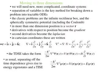
1. Moving to three dimensions • we will need new, more complicated, coordinate systems • separation of variables is the key method for breaking down a problem into tractable ODEs • the classic problems are the infinite rectilinear box, and the spherically symmetric potential (including the Coulomb) • in more than one dimension position is a vectorr • derivatives with respect to position become the gradient • second derivatives become the laplacian • in cartesian coordinates these are written • the TDSE takes the form • as usual, separating off the time dependence gives rise to energy eigenstates and a TISE

2. Expressing this stuff in spherical coordinates (r, q, f) • r is the distance from the origin • qis the polar angle, also called co-latitude: angle down from +z axis; ranges from 0 to p • fis the azimuthal angle : angle away from +x axis in xy plane in counterclockwise sense; ranges from 0 to 2p • the volume element is obtained by increasing each coordinate infinitesimally: • (dr) (r dq ) (r sinq df) = r2 sinqdr dqdf • x = r sinq cos f • y = r sinq sin f • z = r cosq • with s2 = x2 + y2, we have r2 = s2 + z2 so we get • r2 = x2 + y2 + z2 tanq =s/z tanf =y/x

3. Expressing this stuff in spherical coordinates • unit vectors defined as an increase in that coordinate only • because the unit vectors change when taking space derivatives, gradient and laplacian get all mixed up • see Griffith’s E&M text appendix and end-papers for one way to systematically keep track of all the formulas and rules for first and second derivatives • to understand a bit more of the form of the Laplacian, note that the unit vectors are NOT CONSTANT! • the basic issue is that when one dots the gradient into the gradient, the dot products of the unit vectors are just 1 (three ways) or zero (six ways) as usual, but taking their derivatives is NOT zero (in five cases).

4. Issues with getting the Laplacian in sphericals I • simple enough so far… • can you visualize it?? • first three terms… of the gradient dotted into itself:

5. Issues with getting the Laplacian in sphericals II • second three terms… of the gradient dotted into itself:

6. Issues with getting the Laplacian in sphericals III • third three terms… of the gradient dotted into itself:

7. Separating the TISE into an angular and a radial part • assume V(r) =V(r) and separation • insert into TISE; divide by RY; multiply by r2; put r dependence on one side and angular (q,f) dependence on the other side: • since left side depends only on r and right side only on (q,f), both sides are a constant, which we write (weirdly, for now) l(l+1) • we arrive at two distinct DEs (one O and one P), which are…

8. Processing the angular part of the TISE • assume yet another separation into polar and azimuthal factors • the Y functions are spherical harmonics • insert the separated form into the angular equation • calling that constant m2, we arrive at two ODEs…

9. Solving the azimuthal equation • the azimuthal equation is easy to handle • the F function must be periodic with period 2p : F(f +2p) = F(f) • so this is why it made sense to write the constant as m2 • since we allow for ± m anyway, the ± is superfluous • the normalization of this is trivial: • all probabilities with a single m eigenvalue are azimuthally (axially) symmetric!

10. Cracking open the polar equation • the polar equation, like the azimuthal equation, contains no physics, and was familiar to the ancients • it is the Legendre equation, and its solutions are the associatedLegendre polynomials • if m = 0, the solutions are the Legendre polynomials (and of course the spherical harmonics have azimuthal symmetry in that case) • let x = cos q and rexpress things in this language

11. Cracking open Legendre’s equation for m = 0 • it is even in its variable, so solutions will be even or odd • try a power series expansion Q(x) = Sanxn , which yields

12. Cracking open Legendre’s equation for m = 0 • there is an even series or an odd series, but not both • for large n, this roughly settles down to an+2 ~ n/n+2 ~ 1 for large 1 • thus, the ratio test for successive terms may be applied and we see that the ratio is x2 a problem at x = ± 1 •  we must terminate the series so an+2 = 0  l = n = 1,2,3… • in this, we use the Legendre polynomial, whichare given by (another) Rodrigues formula • to keep the solution finite at q = 0 and q = p, l must be a non-negative integer, and m must satisfy the inequality |m|  l because otherwise there is a sign flip in the ODE (see?) and things diverge • solutions are associatedLegendre polynomials

13. Graphs of the Legendre polynomials • notice how they are ‘normalized’ to be unity at x = cos q =1  q = 0 (+z axis) P4 P2

14. Normalizing and calculating expectation values • azimuthally symmetric solutions, so that’s covered • polar solutions are integrated on q angle (from 0 to p often) • in x = cosqlanguage, q = 0 x= 1; q =px= 1, so integration on increasing angle has a sign flip if integrating on increasing x • infinitesimal dx gets sign flip too • to normalize (or any other integral) we can do it either way: • the normalized angular wavefunctions are the spherical harmonics • we will shortly see their intimate connection to angular momentum

15. Example of calculation with the Legendres • generate P31; normalize it; find the angles ‘subtended’ by the ‘collar’; find the probability the particle is in that volume

16. Example of calculation with the Legendres • generate P31; normalize it; find the angles ‘subtended’ by the ‘collar’; find the probability the particle is in that volume

17. Pictures of some orbitals • clockwise from upper left: dzz, dyz, dxz, dxy, dx2-y2 • Example of the p orbital calculation is to come