Download
1 / 18
180 likes | 317 Views
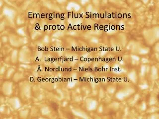
Emerging Flux Simulations & proto Active Regions. Bob Stein – Michigan State U. Lagerfjärd – Copenhagen U. Å. Nordlund – Niels Bohr Inst. D. Georgobiani – Michigan State U. The Simulation.

E N D
Emerging Flux Simulations& proto Active Regions Bob Stein – Michigan State U. Lagerfjärd – Copenhagen U. Å. Nordlund – Niels Bohr Inst. D. Georgobiani – Michigan State U.
The Simulation • Advect minimally structured magnetic field -- horizontal, uniform, untwisted – by inflows at bottom • Complement simulations of coherent, twisted flux tube emergences • Objectives: • Investigate formation and structure of sunspots withoutad hoc boundary conditions • Provide synthetic data for validating local helioseismology and vector magnetograph inversion procedures • Investigate nature of supergranulation
Flux Emergence 20 kG @ 20 Mm depth @ 30o to x-axis, 15 – 32 hrs Average fluid rise time = 32 hrs (interval between frames =1 min) 96 km horizontal resolution -> 48 km Bv Bh
Vertical Magnetic Field Pore/Spot Development (20 kG case) 32.1-35.1 hrs (interval between frames =1 min) Horizontal resolution 24 km.
Emergent Intensity, I/<I> Flux Emergence (20 kG case) 33.3-35.1 hrs (interval between frames =1 min) Horizontal resolution 24 km.
Vertical Velocity (blue/green up, red/yellow down) & Magnetic Field lines (slice at 5 Mm) weak & horizontal B -> normal granulation vertical B -> velocity suppression weak & horizontal B -> normal granulation
Proto-Spot 1 Evolution Flux increase has stopped, ~1x10¹⁹Mx in this spot
Intensity +Bvertical-2.5 blue, -2 green,2 yellow,2.5 red(kG)
Intensity Distribution Active Region Quiet Sun
Velocity Distribution Quiet Sun Active Region
Location of Stokes Data • steinr.pa.msu.edu/~bob/stokes • Simulation results for AR & QS: B, V • Stokes profiles: I,Q,U,V + Hinode annular mtf + slit diffraction + frequency smoothing