Download
1 / 43
440 likes | 740 Views
Measurement Scales. Ar. Aidah Abu Elsoud Alkaissi Link ö ping University. Statistics are either descriptive or inferential. Descriptive statistics: to describe Descriptive and synthesize data. Averages and percentages are examples of descriptive statistics.

E N D
Measurement Scales Ar. Aidah Abu Elsoud Alkaissi Linköping University
Statistics are either descriptive or inferential • Descriptive statistics: to describeDescriptive and synthesize data. Averages and percentages are examples of descriptive statistics. • When such indexes are calculated on data from a population, they are called parameters.
Statistics are either descriptive or inferential • A descriptive index from a sample is called a statistic. Research questions are about parameters, but researchers calculate sample statistics to estimate them, using • inferential statistics to make inferences الاستدلالاتabout the population.
Statistical mean, median, mode, and range The terms mean, median, mode, and range describe properties of statistical distributions.
Mean The most common expression for the mean of a statistical distribution with a discrete random variable is the mathematical average of all the terms. To calculate it, add up the values of all the terms and then divide by the number of terms. This expression is also called the arithmetic mean.
Mean Consider the set of numbers 80, 90, 90, 100, 85, 90. They could be math grades, for example. The MEAN is the arithmetic average, the average you are probably used to finding for a set of numbers - add up the numbers and divide by how many there are: (80 + 90 + 90 + 100 + 85 + 90) / 6 = 89 1/6.
Median The median of a distribution with a discrete random variable depends on whether the number of terms in the distribution is even or odd. If the number of terms is odd, then the median is the value of the term in the middle. This is the value such that the number of terms having values greater than or equal to it is the same as the number of terms having values less than or equal to it. If the number of terms is even, then the median is the average of the two terms in the middle, such that the number of terms having values greater than or equal to it is the same as the number of terms having values less than or equal to it.
Median The MEDIAN is the number in the middle. In order to find the median, you have to put the values in order from lowest to highest, then find the number that is exactly in the middle: 80 85 90 90 90 100 ^ since there is an even number of values, the MEDIAN is between these two, or it is 90. Notice that there is exactly the same number of values ABOVE the median as BELOW it!
Mode The mode of a distribution with a discrete random variable is the value of the term that occurs the most often. It is not uncommon for a distribution with a discrete random variable to have more than one mode, especially if there are not many terms. This happens when two or more terms occur with equal frequency, and more often than any of the others.
Mode The MODE is the value that occurs most often. In this case, since there are 3 90's, the mode is 90. A set of data can have more than one mode
Range The range of a distribution with a discrete random variable is the difference between the maximum value and the minimum value. The RANGE is the difference between the lowest and highest values. In this case 100 - 80 = 20, so the range is 20. The range tells you something about how spread out the data are Data with large ranges tend to be more spread out.
Measurement Scales Variables differ in how well they can be measured, i.e., in how much measurable information their measurement scale can provide. There is obviously some measurement error involved in every measurement, which determines the amount of information that we can obtain. Another factor that determines the amount of information that can be provided by a variable is its type of measurement scale. Specifically, variables are classified as (a) nominal, (b) ordinal, (c) interval, or (d) ratio.
Nominal variables Nominal variables allow for only qualitative classification. That is, they can be measured only in terms of whether the individual items belong to some distinctively different categories, but we cannot quantify or even rank order those categories. For example, all we can say is that two individuals are different in terms of variable A (e.g., they are of different race), but we cannot say which one "has more" of the quality represented by the variable. Typical examples of nominal variables are gender, race, color, city, etc.
Nominal variables • The numeric codes assigned in nominal measurement do not convey quantitative information. • If we classify males as 1 and females as 2, the numbers have no inherent meaning. • The number 2 clearly does not mean “more than” 1. It would be perfectly acceptable to reverse the code and use 1 for females and 2 for males. • The numbers are merely symbols that represent two different values of the gender attribute. • Indeed, instead of numeric codes, we could have used alphabetical symbols, such as M and F.
Nominal measures • Nominal measures must have categories that are mutually exclusive and collectively exhaustive. • For example, if we were measuring ethnicity, we might use the following codes: 1 whites, 2 African Americans, 3 Hispanics. • Each subject must be classifiable into one and only one category.
Nominal measures • The numbers used in nominal measurement cannot be treated mathematically. • We can count elements in the categories, and make statements about frequency of occurrence. • In a sample of 50 patients, if there are 30 men and 20 women, we could say that 60% of the subjects are male and 40% are female. • No further mathematic operations would be meaningful with nominal data.
Example of nominal measures: • Wong, Ho, Chiu, Lui, Chan, and Lee (2002) studied factors contributing to hospital readmission in a Hong Kong hospital. • Their dependent variable (readmission versus not) and several independent variables (e.g., working versus not working, gender, and receives financial assistance or not) were nominal-level variables.
Ordinal variables Ordinal variables allow us to rank order the items we measure in terms of which has less and which has more of the quality represented by the variable, but still they do not allow us to say "how much more. A typical example of an ordinal variable is the socioeconomic status of families. For example, we know that upper-middle is higher than middle but we cannot say that it is, for example, 18% higher. For example, we can say that nominal measurement provides less information than ordinal measurement, but we cannot say "how much less" or how this difference compares to the difference between ordinal and interval scales.
EXAMPLE • Consider a scheme for coding a client’s ability to perform activities of daily living: (1) completely dependent, (2) needs another person’s assistance, (3) needs mechanical assistance, (4) completely independent. • In this case, the measurement is ordinal. • The numbers are not arbitrary—they signify incremental ability to perform activities of daily living. • Individuals assigned a value of four are equivalent to each other with regard to functional ability
Ordinal variables • We do not know if being completely independent is twice as good as needing mechanical assistance. Nor do we know if the difference between needing another person’s assistance and needing mechanical assistance is the same as that between needing mechanical assistance and being completely independent. • Ordinal measurement tells us only the relative ranking of the attribute’s levels. • As with nominal scales, the types of mathematic operation permissible with ordinal-level data are restricted. • Averages are usually meaningless with rank-order measures. • Frequency counts, percentages, and several are appropriate for analyzing ordinal- level data.
Example of ordinal measures: • Bours, Halfens, Abu-Saad, and Grot (2002) studied the prevalence of pressure ulcers in 89 health care institutions in the Netherlands. • Over 15,000 patients were assessed for pressure ulcer severity, using the 4-stage classification of the American and European Pressure Ulcer Advisory Panel. This classification is on an ordinal scale.
Interval variables Interval variables allow us not only to rank order the items that are measured, but also to quantify and compare the sizes of differences between them. For example, temperature, as measured in degrees Fahrenheit or Celsius, constitutes an interval scale. We can say that a temperature of 40 degrees is higher than a temperature of 30 degrees, and that an increase from 20 to 40 degrees is twice as much as an increase from 30 to 40 degrees.
Interval variables • Interval measurement occurs when researchers can specify the rank-ordering of objects on an attribute and can assume equivalent distance between them. • Most psychological and educational tests are based on interval scales. • The Scholastic Assessment Test (SAT) is an example of this level of measurement. • A score of 550 on the SAT is higher than a score of 500, which in turn is higher than 450. • In addition, a difference between 550 and 500 on the test is presumably equivalent to the difference between 500 and 450.
Ratio variables Ratio variables are very similar to interval variables; in addition to all the properties of interval variables, they feature an identifiable absolute zero point, thus, they allow for statements such as x is two times more than y. Typical examples of ratio scales are measures of time or space. For example, as the Kelvin temperature scale is a ratio scale, not only can we say that a temperature of 200 degrees is higher than one of 100 degrees, we can correctly state that it is twice as high.
Ratio variables • The highest level of measurement is ratio measurement. • Ratio scales have a rational, meaningful zero. • Measures on a ratio scale provide information concerning the rank-ordering of objects on the critical attribute, the intervals between objects, and the absolute magnitude of the attribute. • Many physical measures provide ratio-level data. • A person’s weight, for example, is measured on a ratio scale because zero weight is an actual possibility. It is perfectly acceptable to say that someone who weighs 200 pounds is twice as heavy as someone who weighs 100 pounds.
Ratio variables • Because ratio scales have an absolute zero, all arithmetic operations are permissible. • One can meaningfully add, subtract, multiply, and divide numbers on a ratio scale. • All the statistical procedures suitable for interval-level data are also appropriate for ratio-level data.
Example of ratio measures: • Lindeke, Stanley, Else, and Mills (2002) studied academic performance and the need for special services among school-aged children who had been in a level 3 neonatal intensive care unit (NICU). • Numerous ratio-level measures of neonatal characteristics (e.g., birth weight, length at birth, head circumference, and number of days in the NICU) were used to describe the sample and to predict outcomes.
What is "Statistical Significance" (p-value)? The statistical significance of a result is the probability that the observed relationship (e.g., between variables) or a difference (e.g., between means) in a sample occurred by pure chance ("luck of the draw"), and that in the population from which the sample was drawn. The statistical significance of a result tells us something about the degree to which the result is "true" (in the sense of being "representative of the population").
What is "Statistical Significance" (p-value)? The value of the p-value represents a decreasing index of the reliability of a result. The higher the p-value, the less we can believe that the observed relation between variables in the sample is a reliable indicator of the relation between the respective variables in the population. The p-value represents the probability of error that is involved in accepting our observed result as valid, that is, as "representative of the population. " For example, a p-value of .05 (i.e.,1/20) indicates that there is a 5% probability that the relation between the variables found in our sample is a "fluke."
What is "Statistical Significance" (p-value)? Assuming that in the population there was no relation between those variables whatsoever, and we were repeating experiments such as ours one after another, we could expect that approximately in every 20 replications of the experiment there would be one in which the relation between the variables in question would be equal or stronger than in ours. When there is a relationship between the variables in the population, the probability of replicating the study and finding that relationship is related to the statistical power of the design. In many areas of research, the p-value of .05 is customarily treated as a "border-line acceptable" error level.
How to Determine that a Result is "Really" Significant to what level of significance will be treated as really "significant." the selection of some level of significance, up to which the results will be rejected as invalid, is arbitrary. In practice, the final decision usually depends on whether the outcome was predicted a priori or only found post hoc in the course of many analyses and comparisons performed on the data set, on the total amount of consistent supportive evidence in the entire data set, and on "traditions" existing in the particular area of research. Typically, in many sciences, results that yield p .05 are considered borderline statistically significant, but remember that this level of significance still involves a pretty high probability of error (5%). Results that are significant at the p .01 level are commonly considered statistically significant, and p .005 or p .001 levels are often called "highly" significant.
Statistical Significance and the Number of Analyses Performed The more analyses man perform on a data set, the more results will meet "by chance" the conventional significance level. For example, if you calculate correlations between ten variables (i.e., 45 different correlation coefficients), then you should expect to find by chance that about two (i.e., one in every 20) correlation coefficients are significant at the p .05 level, even if the values of the variables were totally random and those variables do not correlate in the population. Some statistical methods that involve many comparisons and, thus, a good chance for such errors include some "correction" or adjustment for the total number of comparisons. many statistical methods (especially simple exploratory data analyses) do not offer any straightforward remedies to this problem. Therefore, it is up to the researcher to carefully evaluate the reliability of unexpected findings.
Example: Baby Boys to Baby Girls Ratio example There are two hospitals: in the first one, 120 babies are born every day; in the other, only 12. On average, the ratio of baby boys to baby girls born every day in each hospital is 50/50. However, one day, in one of those hospitals, twice as many baby girls were born as baby boys. In which hospital was it more likely to happen? The answer is obvious for a statistician, but as research shows, not so obvious : it is much more likely to happen in the small hospital. The reason for this is that technically speaking, the probability of a random deviation of a particular size (from the population mean), decreases with the increase in the sample size
Why Small Relations Can be Proven Significant Only in Large Samples The previous examples indicate that if a relationship between variables in question is "objectively" (i.e., in the population) small, then there is no way to identify such a relation in a study unless the research sample is correspondingly large. Even if our sample is in fact "perfectly representative," the effect will not be statistically significant if the sample is small. if a relation in question is "objectively" very large, then it can be found to be highly significant even in a study based on a very small sample.
Why the "Normal Distribution" is Important The distribution of many test statistics is normal or follows some form that can be derived from the normal distribution. The exact shape of the normal distribution (the characteristic "bell curve") is defined by a function that has only two parameters: mean and standard deviation.
Why the "Normal Distribution" is Important A characteristic property of the normal distribution is that 68% of all of its observations fall within a range of ±1 standard deviation from the mean, and a range of ±2 standard deviations includes 95% of the scores. Symmetric distributions thus consist of two halves that are mirror images of one another. With real data sets, distributions are rarely perfectly symmetric, but minor discrepancies are ignored in characterizing a distribution’s shape. In asymmetric or skewed distributions, the peak is off center and one tail is longer than the other. When the longer tail points to the right, the distribution is positively skewed. Personal income, for example, is positively skewed. Most people have low to moderate incomes, with relatively few people in high-income brackets in the tail. If the tail points to the left, the distribution is negatively skewed,
Figure 2.1 Normal curve calculated from diastolic blood pressures of 500 men, mean 82 mmHg, standard deviation 10 mmHg.
Are All Test Statistics Normally Distributed? Typically, these tests require that the variables analyzed are themselves normally distributed in the population, that is, they meet the so-called "normality assumption. " Many observed variables actually are normally distributed, which is another reason why the normal distribution represents a "general feature" of empirical reality. The problem may occur when we try to use a normal distribution-based test to analyze data from variables that are themselves not normally distributed In such cases, we have two general choices. First, we can use some alternative "nonparametric" test (or so-called "distribution-free test" but this is often inconvenient because such tests are typically less powerful and less flexible in terms of types of conclusions that they can provide. Alternatively, in many cases we can still use the normal distribution-based test if we only make sure that the size of our samples is large enough.
Are All Test Statistics Normally Distributed Namely, as the sample size increases, the shape of the sampling distribution (i.e., distribution of a statistic from the sample; this term was first used by Fisher, 1928a) approaches normal shape, even if the distribution of the variable in question is not normal. This principle is illustrated in the following animation showing a series of sampling distributions (created with gradually increasing sample sizes of: 2, 5, 10, 15, and 30) using a variable that is clearly non-normal in the population, that is, the distribution of its values is clearly skewed.
Why Significance of a Relation between Variables Depends on the Size of the Sample If there are very few observations, then there are also respectively few possible combinations of the values of the variables and, thus, the probability of obtaining by chance a combination of those values indicative of a strong relation is relatively high. illustration. If we are interested in two variables (Gender: male/female and income: high/low), and there are only four subjects in our sample (two males and two females), then the probability that we will find, purely by chance, a 100% relation between the two variables can be as high as one-eighth. Specifically, there is a one-in-eight chance that both males will have a high income and both females a low income, or vice versa.
Standard deviation is a widely used measurement of variability or diversity used in statistics and probability theory. It shows how much variation or "dispersion" there is from the average (mean, or expected value). A low standard deviation indicates that the data points tend to be very close to the mean, whereas high standard deviation indicates that the data are spread out over a large range of values.