Download

1 / 59
620 likes | 912 Views
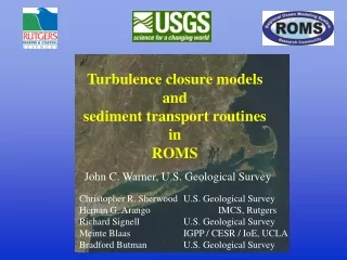
Turbulence closure models and sediment transport routines in ROMS. John C. Warner, U.S. Geological Survey. Christopher R. Sherwood U.S. Geological Survey Hernan G. Arango IMCS, Rutgers Richard Signell U.S. Geological Survey Meinte Blaas IGPP / CESR / IoE, UCLA

E N D
Turbulence closure modelsandsediment transport routinesinROMS John C. Warner, U.S. Geological Survey Christopher R. Sherwood U.S. Geological Survey Hernan G. Arango IMCS, Rutgers Richard Signell U.S. Geological Survey Meinte Blaas IGPP / CESR / IoE, UCLA Bradford Butman U.S. Geological Survey
Outline • Turbulence Closure Models (focus on GLS) • Available models in ROMS • Background of two-equation models • GLS method • Numerical implementation • Applications • Open channel flow(2) • Surface mixed layer deepening • Estuary (idealized + realistic) • Sediment Transport Routines • Overview of routines • Applications • Summary
Reynolds Averaged Navier Stokes Equations Continuity Momentum Transport Equation of State unknowns u, v, w, h, temp, sal, ssc,
Available turbulence closures in ROMS • Background value • Analytical expression • BVF - Brunt_Vaisala frequency • LMD - Large / McWilliams / Doney • Two equation models: • MY25 - Mellor/Yamada 2.5 • GLS - Umlauf/Burchard Generic Length Scale
Available turbulence closures in ROMS • Background value • ocean.in ! Vertical mixing coefficients for active tracers: [1:NAT,Ngrids] AKT_BAK == 5.0d-6 5.0d-6 ! m2/s ! Vertical mixing coefficient for momentum: [Ngrids]. AKV_BAK == 5.0d-6 ! m2/s • mod_mixing.F DO itrc=1,NAT MIXING(ng) % Akt(Imin:Imax,Jmin:Jmax,1:N(ng)-1,itrc) = & & Akt_bak(itrc,ng) END DO MIXING(ng) % Akv(Imin:Imax,Jmin:Jmax,1:N(ng)-1) = Akv_bak(ng)
Available turbulence closures in ROMS • Analytical • cppdefs.h #define ana_vmix • analytical.F, ana_vmix # elif defined SED_TEST1 DO k=1,N(ng)-1 ! vonkar*ustar*z*(1-z/D) DO j=JstrR,JendR DO i=IstrR,IendR Akv(i,j,k)=0.025_r8*(h(i,j)+z_w(i,j,k))* & & (1.0_r8-(h(i,j)+z_w(i,j,k)) / (h(i,j)+zeta(i,j,knew))) Akt(i,j,k,itemp)=Akv(i,j,k)*0.49_r8/0.39_r8 Akt(i,j,k,isalt)=Akt(i,j,k,itemp) END DO END DO END DO
Available turbulence closures in ROMS • BVF • !----------------------------------------------------------------------- • ! Set tracer diffusivity as function of the Brunt-vaisala frequency. • ! Set vertical viscosity to its background value. • !----------------------------------------------------------------------- • cppdefs.h • #define BVF_MIXING /* Activate Brunt-Vaisala frequency mixing */
Available turbulence closures in ROMS • LMD • cppdefs.h /* Options for the Large/McWilliams/Doney interior mixing */ # define LMD_MIXING #undef LMD_SKPP /* surface boundary layer KPP mixing */ #undef LMD_BKPP /* bottom boundary layer KPP mixing */ #undef LMD_NONLOCAL /* nonlocal transport */ #undef LMD_RIMIX /* diffusivity due to shear instability */ #undef LMD_CONVEC /* convective mixing due to shear instability */ #undef LMD_DDMIX /* double-diffusive mixing */
Available turbulence closures in ROMS Two Equation Models • MY25 • cppdefs.h #define MY25_MIXING • GLS • cppdefs.h #define GLS_MIXING • For either MY25 or GLS • cppdefs.h #define KANTHA_CLAYSON or #define CANUTO_A or #define CANUTO_B #define N2S2_HORAVG
Transport equation for Reynolds Stresses Reynolds Stress transport Pressure-strain correlation 1 3 Pij Wij Bij Pij 1 eij 2 dissipation 2 Triple correlation 3
Transport equation for Reynolds Stresses:scaled + boundary layer approximation Pij Wij Bij Scaling by q3/L BL: - neglect rotation - neglect gradients parallel to boundary Pij eij
Parameter A1 A2 B1 B2 C2 C3 Value 0.92 0.74 16.6 10.1 0.7 0.2 Algebraisation of second moment clsoures:eddy viscosity and diffusivity “k” “e” notation or “q” “l” notation eddy viscosity eddy viscosity eddy diffusivity eddy diffusivity Table 2. Kantha and Clayson (1994) stability function parameters So now need 2 equations: one for q (or k) one for l (or e)
Two equation turbulence closures MY25 (Mellor, Yamada 1982) k - e (Rodi, 1980) k - w (Wilcox, 1988)
Why does MY25 need a wall proximity function? assume st st, no horiz grad, no B where in bottom constant stress layer : l = k z, P = e, q2 is const Negative diffusion without a wall function E1 = 1.8 B1 =16.6 E2 = 1.33 Sq = 0.2
Umlauf and Burchard (2003) J. Mar. Res. “Generic Length Scale” turbulence closure p, m, n : define y sk: diffusion of k sy: diffusion of y, fit to law of wall c1: homogenous sheared grid turbulence c2: free decay of homogenous turbulence c3: buoyancy parameter for unstable Warner, Sherwood, Arango, and Signell (2005) Performance of four turbulence closure models implemented using a generic length scale method, Ocean Modelling 8, p. 81-113.
Determination of c3 buoyancy coefficient Start with transport equation for y Assume: P + B = e Substitute expressions for KM, B, and e can derive: length scale limitation l < sqrt (0.56 k) / N yields: for Kantha/Clayson stability functions
Numerical implementationgrid + limitations k (q2) limitation: k = MAX(k, 1e-8) Length scale limitation:
Numerical implementation MY25 GLS 1 time step advective transport terms time step with P, B time step e (F) apply BCs, time step diff term, update values calc length scale calc buoyancy parameter Gh = ( L N / Q) ^2 limit Gh calc stability functions Sm, Sh = functs (Gh) calc eddy visc and eddy diff Km = Q L Sm, Kh = Q L Sh, Kq = Q L Sq ; wall fnct (l). 2 3 k, y at new time step q2, q2l at new time step
Test Cases • Open channel flow (2 simulations) to compare closures with velocity log layer 2) Mixed layer deepening to calibrate c3 buoyancy parameter 3) Estuary
h Q Test Case # 1: Steady Open Channel Flow:Experimental Description Domain parameters L = 10000, W=1000, H=10 m Zob = 0.005 ubar = 1m/s S0 = 4x10⁻⁵ m/m tcr = 0.05 N/m2 E = 5x10⁻⁵ kg/m2/s Porosity = 0.90 2 simulations Model parameters 1) h and Q z grid spacings: dx = 100m, dy = 10m, dz = 0.25m) dt = 30s 5000 s simulated (st. st. reached) x h h 2) h and h Q
Test Case # 1: Steady Open Channel Flow:Analytical Results momentum eq. linear stress shear velocity velocity eddy viscosity turbulent kinetic energy = 0.013 m2/s2 at z = 0
Test Case # 1: Steady Open Channel Flow Simulation 1 Depth and Flow h Q
Test Case #2 : Surface mixed layer deepening Means to confirm c3 buoyancy parameter z x z Domain parameters r L = 5000, W=1000, H=50 m Zos = 0.005 u*surf = 0.01 m/s N0 = 0.01 /s Dm Model parameters grid spacings: dx = 250m, dy = 100m, dz = 0.25m) dt = 30s 30 days simulated
Test Case #2 : Surface mixed layer deepening Mixed layer depth, Dm (Price, 1979) Critical Richardson No. controls evolution of mixed layer deepening
Test case #3 : Idealized estuary Domain parameters L = 100000, W=1000, H=5-10 m Zob = 0.005 River ubar = 0.08m/s Tidal ubar = 0.40 m/s S0 = 5x10⁻⁵ m/m tcr = 0.05 N/m2 ws = 0.5mm/s E = 1x10⁻⁴ kg/m2/s Porosity = 0.90 Model parameters grid spacings: dx = 500m, dy = 100m, dz = 0.25-0.5 m dt = 30s 20 days (~st. st. reached)
Test case #3 : Idealized estuary Domain parameters L = 100000, W=1000, H=5-10 m Zob = 0.005 River ubar = 0.08m/s Tidal ubar = 0.40 m/s S0 = 5x10⁻⁵ m/m tcr = 0.05 N/m2 ws = 0.5mm/s E = 1x10⁻⁴ kg/m2/s Porosity = 0.90 Model parameters grid spacings: dx = 500m, dy = 100m, dz = 0.25-0.5 m dt = 30s 20 days (~st. st. reached)
Realistic estuary - Hudson River John C. Warner W. Rockwell Geyer James A. Lerczak 200 along channel cells 20 lateral cells 20 vertical levels
Model parameters Initial parameters Initial salinity distribution level free surface zero velocity salt distribution Operational parameters dt = 30s z0 = 0.005 Simulate: - tides, salt, suspended-sediment - for 50 days (days 100 – 150 , 2003)
Boundary conditions • Northern end: • Measured Q • Salinity = 0 • Southern end: • Tidal boundary using observed free surface only • Salinity gradient condition salbndry = salj=1+ dSdx
Comparison of vertical structure of salt and velocity (k-w) Observed Neap tide Model Observed Spring tide Model
BBL and Sediment • Bottom boundary layer subroutines - enhance bottom stress to include the average affect of surface waves on the mean currents (mb_bbl.F and sg_bbl.F) • Sediment transport subroutine – transport multiple classes of suspended sediment and track evolution of multi-layered bed framework (sediment.F) • User can specify : • 1) just BBL • 2) just Sediment • 3) or both BBL + Sediment
Non-linear enhancement wave-mean bottom stress tmean/(tcurrent+twave) tcurrent/(tcurrent+twave) Wave - Current BBL Physics • Increased turbulence • Enhanced drag • Enhanced mean stress • Increased maximum stress • Moveable bed roughness • Input: • Current speed and direction at reference height • Wave orbital velocity, period, and direction • Bottom sediment characteristics • Output: • Apparent drag coefficient • Wave-maximum shear stress • Bedform geometry Grant and Madsen (1986) Ann. Rev. Fluid Mech. 18:265-305
SG_BBL Modifed Grant-Madsen w-c model (Styles & Glenn, 2000) Formally related to three-layer eddy viscosity profile Ripple roughness (Styles & Glenn, 2000) Immobile sediment roughness gets default value No skin friction / form drag partitioning; no sediment stratification Contributed by Rich Styles and Scott Glenn MB_BBL Empirical DATA2 wave-current solution (Soulsby, 1995) Ripple geometry for sand or silty beds Nikuradse, saltation, ripple, and/or biogenic roughness (Combination of methods) Faster than SG_BBL No skin friction / form drag partitioning; no sediment stratification Contributed by Meinte Blass W-C Bottom Boundary Layer Routines
waves data: SWAN.nc, ana_waves T, Dir, Amp / Ub model “flow chart” bottom drag: ocean.in rdrg rdrg2 Zo #if defined bbl_model #else sg_bbl.F mb_bbl.F set_vbc.F bustr, bustrcwmax bvstr, bvstrcwmax bottom(i,j, irlen) irhgt) bustr bvstr surficial sed data: ana_sediment, forcing.nc, or sediment.F bottom(i,j, isd50) idens) iwsed) itauc) hydrodynamic routines (advection-diffusion) #if defined sediment #else sediment.F (deposition and erosive fluxes, bed evolution) sediment data: ana_sediment or initial.nc bed (i,j,k, thick) botom(i,j, isd50) age) idens) poro) iwsed) diff) itauc) bed_frac(i,j,k,ised) irlen) bed_mass(i,j,k,ised) irhgt) izdef) ….. )
Sediment transport – bed layers Erosion Active layer thick Harris, Wiberg 1997 Deposition Rule: create a new layer for deposition if top layer > 5mm Active layer thick
Example application : Massachusetts Bay http://pubs.usgs.gov/of/2003/of03-001/index.htm multibeam backscatter intensity Surficial sediment characteristics Surficial mean grain size distribution- binned 2:6
Wentworth grade scale Phi Initial conditions: 5 sediment classes 8 bed layers (5 cm ea.) Equal fractions 2 3 4 5 6 http://pubs.usgs.gov/of/2003/of03-001/htmldocs/nomenclature.htm
Sed particle property calcs Google: Sherwood USGS + other Sediment transport applets http://woodshole.er.usgs.gov/staffpages/csherwood/sedx_equations/RunSedCalcs.html
activate sediment and bbl cppdefs.h activate sediment activate bbl activate source of wave data
specify input file and output parameters ocean.in activate output identify name of sediment.in file
Establish sediment parameters mod_param.F set grid size set : number of bed layers number of cohesive sediment classes number of non-cohesive sediment classes
Initialize sediment arrays ana_sediment bed(i,j,k, MBEDP) ithck = 1 ! layer thickness iaged = 2 ! layer age iporo = 3 ! layer porosity idiff = 4 ! layer bio-diffusivity bed_frac(i,j,k, ised) bed_mass(i,j,k, ised) bottom(i,j, MBOTP) isd50 = 1 ! mean grain diameter idens = 2 ! mean grain density iwsed = 3 ! mean settle velocity itauc = 4 ! critical erosion stress irlen = 5 ! ripple length irhgt = 6 ! ripple height ibwav = 7 ! wave excursion amplitude izdef = 8 ! default bottom roughness izapp = 9 ! apparent bottom roughness izNik = 10 ! Nikuradse bottom roughness izbio = 11 ! biological bottom roughness izbfm = 12 ! bed form bottom roughness izbld = 13 ! bed load bottom roughness izwbl = 14 ! wave bottom roughness iactv = 15 ! active layer thickness ishgt = 16 ! saltation height
Modeling of sediment transport in Mass Bay Justification: • Relocation of Boston sewage outfall (Sept 2000) • Habitats – fisheries Purpose • simulate tidal currents and transport of sediment due to combined tides and storm forcing • determine transport pathways of sediment in Mass Bay (relative contribution of storms, tides, etc) • test of numerical transport algorithms, bed model Methods • Conduct 70 day simulation of currents and sediment transport, driven by tides and 6 repeating storm events Butman, Valentine http://woodshole.er.usgs.gov/project-pages/coastal_mass/html/intro.html
Grid 20 vertical sigma layers68x68 horizontal orthogonal curvilinear