Phylogenetics
Phylogenetics. “Inferring Phylogenies” Joseph Felsenstein Excellent reference. What is a phylogeny?. Different Representations. Cladogram - branching pattern only Phylogram - branch lengths are estimated and drawn proportional to the amount of change along the branch

Phylogenetics
E N D
Presentation Transcript
Phylogenetics “Inferring Phylogenies” Joseph Felsenstein Excellent reference
Different Representations • Cladogram - branching pattern only • Phylogram - branch lengths are estimated and drawn proportional to the amount of change along the branch • Rooted - implies directionality of change • Unrooted - does not • How do you root a tree?
Estimate a Phylogeny Sp1 ACCGTCTTGTTA Sp2 AGCGTCATCAAA Sp3 AGCGTCATCAAA Sp4 ACCGTCTTGATA Sp5 AGCCTCTTCATA
Estimate a Phylogeny Sp1 ACCGTCTTGTTA Sp2 AGCGTCATCAAA Sp3 AGCGTCATCAAA Sp4 ACCGTCTTGATA Sp5 AGCCTCTTCATA
Working Tree sp2 sp1 c2 sp3 sp5 sp4
Estimate a Phylogeny Sp1 ACCGTCTTGTTA Sp2 AGCGTCATCAAA Sp3 AGCGTCATCAAA Sp4 ACCGTCTTGATA Sp5 AGCCTCTTCATA
Working Tree sp2 sp1 c2 sp3 c4 sp5 sp4
Estimate a Phylogeny Sp1 ACCGTCTTGTTA Sp2 AGCGTCATCAAA Sp3 AGCGTCATCAAA Sp4 ACCGTCTTGATA Sp5 AGCCTCTTCATA
Working Tree sp2 sp1 c7 c2 sp3 c4 sp5 sp4
Estimate a Phylogeny Sp1 ACCGTCTTGTTA Sp2 AGCGTCATCAAA Sp3 AGCGTCATCAAA Sp4 ACCGTCTTGATA Sp5 AGCCTCTTCATA
Working Tree sp2 sp1 c7 c2 sp3 c4 c9 sp5 sp4
Estimate a Phylogeny Sp1 ACCGTCTTGTTA Sp2 AGCGTCATCAAA Sp3 AGCGTCATCAAA Sp4 ACCGTCTTGATA Sp5 AGCCTCTTCATA
Working Tree sp2 sp1 c10 c7 c2 sp3 c4 c9 sp5 sp4
Estimate a Phylogeny Sp1 ACCGTCTTGTTA Sp2 AGCGTCATCAAA Sp3 AGCGTCATCAAA Sp4 ACCGTCTTGATA Sp5 AGCCTCTTCATA
Final Tree sp2 sp1 c10 c11 c2 c7 sp3 c4 c9 sp5 sp4
What optimality criteria do we use then? • Parsimony • Likelihood • Bayesian • Distance methods?
Parsimony • Why should we choose a specific grouping? • Maximum parsimony: we should accept the hypothesis that explain the data most simply and efficiently • “Parsimony is simply the most robust criterion for choosing between competing scientific hypotheses. It is not a statement about how evolution may or may not have taken place”1 1 Kitching, I. J.; Forey, P. L.; Humphries, J. & Williams, D. M. 1998. Cladistics: the theory and practice of parsimony analysis. The systematics Association Publication. No. 11.
Parsimony • Optimality criteria that chooses the topology with the less number of transformations of character states • Optimizing one component: tree topology (pattern based) • Most parsimonious tree: the one (or multiple) with the minimum number of evolutionary changes (smaller size/tree length)
A O C D B 6. T=>G 6. T=>G 5. A=> GAP 2. G=>A 4. A=>C 3. T=>C 4. A=>G 1. T=>A Reconstructing trees via sequence data Tree length = 8
Models of Evolution T C Pyrimidines A G Purines Transversions Transitions
Maximum Likelihood • Base frequencies: fA + fG + fC + fT = 1 • Base exchange: fs + fv = 1 • R-matrix: + + + + + = 1 • Gamma shape parameter • Number of discrete gamma-distribution categories • Pinvar: fvar + finv = 1 • Likelihood: L = li where i is each character state
Maximum Likelihood C G G t4 t5 A G y t2 t1 t3 t6 x z • L=Pr(D|H) t7 t8 w
ML cont. the probability that the nucleotide at time t is i is given by the probability that the nucleotide at time t is j, ji, is given by
Prob (H) Prob (D│H) Prob (H │D) = Prob (D) Bayes Theorem Prior probability or Marginal probability of H The conditional probability of H given D: posterior probability Likelihood function H=Hypothesis D=Data Prior probability or Marginal probability of D ∑HP(H) P(D|H) Normalizing Constant: ensures ∑ P (H │D) = 1
Take Home Message • Likelihood: represents the P of the data given the hypothesis => difficult to interpret • Bayes approach: estimates the P of the hypothesis given the data => estimates P for the hypothesis of interest
f(i) f(X|i) f(i |X) = B(s) ∑j=1 f(i) f(X|i) f(i,i,) f(X|i,i,) f(i,i,|X) = B(s) ∑j=1 ∫ ,f(i,i,) f(X| i,i,)dd ∫ , f(i,i,) f(X|i,i,) dd f(i|X) = B(s) ∑j=1 ∫ , f(i,i,) f(X| i,i,)dd Bayesian Inference of Phylogeny • Calculating pP of a tree involves a summation over all possible trees and, for each tree, integration over all combinations of bl and substitution-model parameter values • Inferences of any single parameter are based on the marginal distribution of the parameter • This marginal P distribution of the topology, for example, integrates out all the other parameters • Advantage: the power of the analysis is focused on the parameter of interest (i.e., the topology of the tree)
Estimating phylogenies • Exhaustive Searches • Branch and bound methods • Rise in computational time versus rise in solution space
HIV-1 Whole Genomes 1993 - 15 HIV-1 Whole Genomes 2003 (JAN) - 397
Heuristic Searches • Nearest-neighbor interchanges (NNI) - swap two adjacent branches on the tree • Subtree pruning and regrafting (SPR) - removing a branch from the tree (either an interior or an exterior branch) with a subtree attached to it. The subtree is then reinserted into the remaining tree in all possible places • Tree bisection and reconnection (TBR) - An interior branch is broken, and the two resulting fragments o the tree ar considered as separate trees. All possible connections are made between a branch of one and a branch of the other.
Other approaches • Tree-fusing - find two near optimal trees and exchange subgroups between the two trees • Genetic Algorithms - a simulation of evolution with a genotype that describes the tree and a fitness function that reflects the optimality of the tree • Disc Covering - upcoming paper
Phylogenetic Accuracy? • Consistency - A phylogenetic method is consistent for a given evolutionary model if the method converges on the correct tree as the data available to the method become infinite. • Efficiency - Statistical efficiency is a measure of how quickly a method converges on the correct solution as more data are applied to the problem. • Robustness - Robustnessrefers to the degree to which violations of assumptions will affect performance of phylogenetic methods
How reliable is MY phylogeny? • Bootstrap Analysis • Jackknife Analysis • Posterior Probabilities (Bayesian Approaches) • Decay Indices