Phylogenetics
Phylogenetics. 3/2/2018. Acknowledgements. Much of the content of this lecture is from:. Yang (2012) – Molecular phylogenetics principles and practices. What is phylogenetics?. Study of evolutionary history among groups of organisms. Phylogenetics and Bioinformatics.


Phylogenetics
E N D
Presentation Transcript
Phylogenetics 3/2/2018
Acknowledgements Much of the content of this lecture is from: • Yang (2012) – Molecular phylogenetics principles and practices
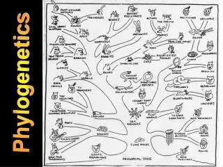
What is phylogenetics? Study of evolutionary history among groups of organisms
Phylogenetics and Bioinformatics • A foundational topic in bioinformatics • Subject of research in 1980s and 1990s as DNA sequences became more available • Renewed interest now with NGS and the explosion of sequencing data • Phylogenetics itself has been around for hundreds of years…
Taxonomy • History of phylogenetics is rooted in taxonomy • Taxonomy: defining and naming organisms based on shared characteristics • A basic taxonomy has likely always been in place
Pre-Linnaean Taxonomy • Egyptian paintings from ~1500 BC depict plants with medicinal properties • Aristotle (384-322 BC) classified animals based on attributes (number of legs, laying eggs, warm-bodied, etc.) • Bhagavata Purana (Hindu texts from 500-1000 CE) explicitly defines 6 sub-types of plants (large trees with and w/o fruits, small plants, bushes) • Andrea Cesalpino (1519-1603), the “first taxonomist”, formally describes ~1500 plant species in 1583
Carl Linnaeus (1707-1778) • Swedish botanist, zoologist, physician • Systema Naturae(1735) established three “kingdoms” – animal, vegetable, and mineral • We still use hierarchy described in the 10th edition (1758) – kingdoms, classes, orders, genera, species • Popularized use of binomial nomenclature (eg. Homo sapiens) • 1st edition: 11 pages - whales are fish • 10th edition: 1,300 pages - whales are mammals
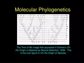
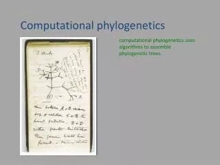
From taxonomy to phylogenetics • Phylogenetics is taxonomy but applied to theory of evolution • Related species in these classifications have a common ancestor • Charles Darwin used a tree to illustrate evolution, ancestors in On the Origin of Species (1859) • Darwin’s notes from 1837 show his first tree sketch
Molecular Phylogenetics • Today, bioinformatics uses sequencing data to study phylogenetics (instead of observable traits) • Molecular phylogenetics leverages similarities and differences between DNA sequences to gain information on evolutionary relationships
Molecular Phylogenetics GOAL: examine and visualize relationships between a group of species or DNA elements within a species (gene paralogs) using DNA sequences themselves
Applications of Phylogenetics • Origin and spread of a viral infection • Genealogical relationship between cells during cancer development • Origin and relationship between paralogs of a gene • Migration patterns of a species • Evolution of language • Classification of metagenomics samples • Annotation of newly sequenced genomes • Reconstruction of ancestral genomes
This Lecture • Basic phylogenetic tree concepts • Strategies and methodologies for tree reconstruction • Assessment of phylogenetic methods • Some commonly used phylogenetics tools
Phylogenetic Tree Terminology clade Taxon (OTU) Branch (lineage) Internal Node (shared ancestor) Terminal node Root outgroup Branch Length (time)
The Phylogenetic Tree as a Model • Nodes 1, 2, and 3 are separated by 2 speciation events at T0 and T1 • Branch lengths (b) are units of substitution and measure evolution over time • If substitution rate is constant: b0 + b1 = b0 + b2 = b3
Rooted Tree vs. Unrooted Tree • If each branch length has independent evolutionary rate, unable to identify root • Common strategy is to include an outgroup to root the tree
Phylogenetic Tree Reconstruction • For molecular phylogenetics, you start with some group of DNA, RNA, or protein sequences • You first need to perform a multiple sequence alignment (MSA) • Tree reconstruction based on MSA can either be done using distance-based or character-based methods
DNA Sequence Alignment (Redux) Sequence 1 ATACACAGTAGGAGATACCAGTAAGGGAGGGGG Sequence 2 ATACCATAAGCGAG Match Mismatch ATACACAGTAGGAGATACCAGTAAGGGAGGGGG --------------ATACCA-TAAGCGAG---- Alignment 1 Gap ATACACAGTAGGAGATACCAGTAAGGGAGGGGG ATAC-CA--------------TAAGCGAG---- Alignment 2 Alignment 3 ATACACAGTAGGAGATACCAGTAAGGGAGGGGG ATAC-CA-TA--AG---C--G--AG--------
Scoring/Substitution Matrices • Given alignment, how “good” is it? • Higher score = better alignment • Implicitly represent evolutionary patterns ATACCAGTAAGGGAG ATACCA-TAAGAGAG Score = 22 ATACCAGTAAGG-GAG ATACCA-TAAG-AGAG Score = 19 ATACCA-GTAAGGGAG A-TACCATAAGAGAG- Score = -20
Multiple Sequence Alignment Like pairwise alignment, but with N sequences
Obtaining a Multiple Sequence Alignment • Example using ClustalW2 • Input: group of FASTA sequences • Output: Clustal format alignment * = identical : = conserved . = semi-conserved
Methods for Tree Reconstruction Character-based methods • Maximum parsimony • Maximum likelihood • Bayesian methods Distance-based methods • UPGMA/WPGMA • Neighbor joining • Least squares
Distance-based methods • Use your obtained multiple sequence alignment to compute distances between sequences • Pairwise distances are measured using a substitution matrix (as with scoring alignments) • Pairwise distances between all sequences in your MSA generate a distance matrix
Computing distances • Different substitution models exist • Example: JC69 (Jukes-Cantor) • Model scores every substitution equally • Identical nucleotides at given position scored 0
Different Substitution models • Size of circles = relative proportion of given nucleotide • Thickness of arrow = relative substitution rate
Distance Matrix Example • Given 5 arbitrary sequences – A, B, C, D, and E • Computing pairwise distances using a substitution model generates a 5x5 matrix • Distance matrix can be used to construct a tree
WPGMA Example • Weighted Pair Group Method with Arithmetic Mean • Start with initial pairwise distance matrix A B C • A and B are closest • Join them and compute new distances D E
WPGMA Example • A and B are merged into AB • Distance from AB to C, D, and E are computed A B C • D and E are now closest • Join them and compute new distances D E
WPGMA Example • D and E are merged to DE • Distance from DE to C and AB are computed A B C • C and DE are now closest • Join them and compute new distances D E
WPGMA Example • C and DE are merged into CDE • Distance from CDE to AB is computed A B C • Join final 2 clusters D E
WPGMA Example A B C D • Distances between clusters used to plot rooted tree • Assumes constant evolutionary rate E
Neighbor joining • Initialized with a star network • Iteratively joins nearest taxa, assigning internal nodes • Results in an unrooted tree • Does not assume lineages evolve at same rate
Distance-based methods Strengths: • SPEED and computational efficiency • NJ is good for large data sets with low levels of sequence divergence Weaknesses: • Loss of information (condensing MSA) • No attempts to define internal ancestral nodes
Character-based methods Maximum parsimony • Attempts to find most parsimonious tree • This is the tree that relates the sequences with the least number of mutations Mutations only
Finding the most parsimonious tree • Not exactly an easy task • The number of unrooted trees with n taxa is:
Maximum Likelihood • Likelihood: conditional probability of observing the sequences given a model of evolution and a tree • We’re trying to find the tree and branch lengths that maximize the likelihood function
Maximum Likelihood • Assuming independent substitution rates:
Maximum Likelihood • Likelihoods typically calculated from leaves to root (Felsenstein’s pruning algorithm) • In practice, impossible to visit every tree
Assessing tree topology • Most common way to assess confidence in a tree topology for both distance-based and character-based analyses is the bootstrap analysis • Bootstrapping – number of sites in the MSA are resampled with replacement as many times as the sequence length, generating a pseudo-sample • For each clade in tree, bootstrap support value is proportion of trees that include that clade
Assessing reconstruction methods • Consistency – parameter values converge with increasing data • Efficiency – probability of recovering correct tree given the number of sites in comparison (estimated by simulation) • Robustness – gives correct answers even when assumptions are violated or relaxed • Speed / computational efficiency