Download
1 / 47
470 likes | 588 Views
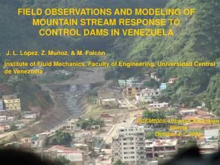
FIELD OBSERVATIONS AND MODELING OF MOUNTAIN STREAM RESPONSE TO CONTROL DAMS IN VENEZUELA. J. L. López, Z. Muñoz, & M. Falcón Institute of Fluid Mechanics, Faculty of Engineering, Universidad Central de Venezuela. RCEM2005, Urbana-Champaign Illinois October 4-7, 2005. Outline.

E N D
FIELD OBSERVATIONS AND MODELING OF MOUNTAIN STREAM RESPONSE TO CONTROL DAMS IN VENEZUELA J. L. López, Z. Muñoz, & M. Falcón Institute of Fluid Mechanics, Faculty of Engineering, Universidad Central de Venezuela RCEM2005, Urbana-Champaign Illinois October 4-7, 2005
Outline • Field observations at Galipan Experimental Basin • A mathematical model to predict bed elevation response to control dams • Some testing cases Case 1. Degradation downstream from a dam Case 2. Aggradation upstream from a dam • Preliminary Application to Macuto Dam
December 1999 1998 1999 The town of Macuto (The San Jose de Galipan Basin)
Macuto Macuto San Jose San Jose Manzanares Picacho G. S Francisco S Isidro Humboldt Los Venados San Jose de Galipan Experimental Basin SJG Hidro Area: 14 km2 Highest elevation 2,300 m Alluvial fan slope: 6 % Main stream length:8.7 km Main stream slope: 52%
Macuto Dam (Galipan river) January, 2004
Macuto Dam (Galipan river) January 2005 February 2005
Flood hydrograph for the significant storms in the San Jose de Galipan basin between March 2003 and January 2005.
Rainfall measurements in Feb. 2005 (stations in the Galipan Experimental Basin)
Landslides and rock fall along the coastal road in Vargas, Feb. 2005
Sedimentation of bridges and chanels San Julián River bridge San Julián River channel Guanape River bridge Camuri River
Sedimentation of dams Quebrada Curucuti Quebrada El Cojo
A MATHEMATICAL MODEL TO PREDICT EROSION AND SEDIMENT DEPOSITION IN MOUNTAIN RIVERS
THE MATHEMATICAL MODEL Steady state flow equation for a constant discharge: Friction factor: Aguirre-Pe et al (1992) for d/D less than 10: Sediment Discharge: Schoklitsch-type equation (1987)
Incipient Motion Condition: Aguirre-Pe and Fuentes R. (1993) Sediment Continuity Equation:
RIVER BED 2Dm 3 2Dmax 1 4 Z ZINF ZS 2 BED ROCK CONTROL Calculation of grain size distribution changes The sediment model considers two layers in the bed. 1. ACTIVE LAYER OR MIXING LAYER 2. SUBSURFACE LAYER 3. UPPER MIXING LAYER 4. LOWER MIXING LAYER Fig. 1. Definition diagram for bed layers
Probability density function fi(Dj) Dmin D1 Dj Dmax,i Dmax Dn+1 Dcr,i Density function of eroded material: Dmin≤ D ≤ Dcr,i for Density function of non-eroded material: for Dcr,i≤ D ≤ Dmax,i
The cumulative grain size distribution function are, respectively: The total volume of sediment contained in the mixing layer of thickness Em is:
Similarly, the volume for any sediment fraction Dj in the mixing layer is: The new sediment fraction in weight of the bed material contained in the mixing layer at time t+Δt is then obtained by dividing the last two expressions:
By definition, the accumulative grain size distribution is given by: Then, integrating the above expression: If the mixing layer becomes very small, what is left of it is mixed with the sub layer material and the temporal process continues.
Computational Procedure At each time step: • Input the flow discharge and boundary conditions. • Calculate the water profile using friction factors for mountain streams • Calculate the initial grain size distribution of bed material. • Calculate the sediment transport by Schoklitsch equation • Determine the critical diameter • Calculate the sediment fractions to be eroded from the bed • Determine the changes in bed elevations • Calculate the grain size distribution changes
STUDY CASE • Degradation downstream from a dam (clear water release). • So = 4 % • River reach L = 2000 m • Rectangular sections B = 25 m • 41 cross sections (space interval=50 m) • Constant flow discharge Q = 200 m3/s • Boulders up to 0.85 m (Dmax = 0,85 m) • Initial circular grain size distribution • Dm = 0.18 m
Degradation downstream from a dam (clear water release). Changes in bed profiles with time So = 4%
Computed time variation in grain size distribution at x = 1800 m (200 m downstream of the dam).
Computed time variation in grain size distribution at x = 1800 m ( 200 m downstream of the dam).
Computed time variation in grain size distribution at x = 1800 m (200 m downstream of the dam).
Computed time variation in grain size distribution at x = 1800 m (200 m downstream of the dam).
Computed time variation in grain size distribution at x = 1800 m (200 m downstream of the dam).
Computed time variation in grain size distribution at x = 1800 m (200 m downstream of the dam).
Computed time variation in grain size distribution at x = 1800 m (200 m downstream of the dam).
Computed time variation in grain size distribution at x = 1800 m (200 m downstream of the dam).
Aggradation upstream from a dam Changes in bed profiles with time
Computed time variation in grain size distribution at a section just upstream of the dam.
Computed time variation in grain size distribution at a section just upstream of the dam.
Computed time variation in grain size distribution at a section just upstream of the dam.
Computed time variation in grain size distribution at a section just upstream of the dam.
Computed time variation in grain size distribution at a section just upstream of the dam.
Computed time variation in grain size distribution at a section just upstream of the dam.
CONCLUSIONS • The sediment control dams in the State of Vargas are being subjected to a very rapid process of sedimentation, due to the large sediment yield capacity of the basins. • The numerical model is able to reproduce alternate processes of coarsening and refining of bed material and simulates the general tendency of the armoring process. • Preliminary application of the model to Macuto Dam show that the Shoklitsch equation underestimate the sediment transport capacity of the stream. Further work is needed to investigate the effect of the mixing layer thickness in the evolution of the river bed.
XXII Latin American Congress on HydraulicsInternational Symposium on Hydraulic Structures (IAHR Hydraulic Structures Section)October 9-14, 2006 in Ciudad Guayana, Venezuela Ciudad Guayana
THANKS FOR YOUR ATTENTION Ciudad Guayana