Download
1 / 1
20 likes | 232 Views
COMBINED MODELING OF THE EARTH’S GRAVITY FIELD FROM GOCE AND GRACE SATELLITE OBSERVATIONS Robert Tenzer 1 , Pavel Ditmar 2 , Xianglin Liu 2 , Philip Moore 1 , Roland Klees 2

E N D
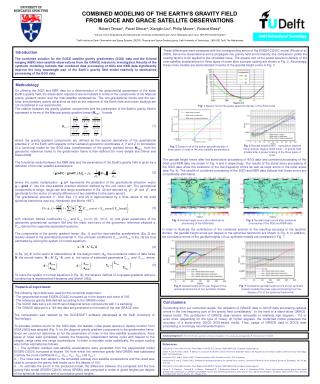
COMBINED MODELING OF THE EARTH’S GRAVITY FIELD FROM GOCE AND GRACE SATELLITE OBSERVATIONS Robert Tenzer1, Pavel Ditmar2, Xianglin Liu2, Philip Moore1, Roland Klees2 1 School of Civil Engineering and Geosciences, University of Newcastle upon Tyne, Newcastle upon Tyne, NE17RU United Kingdom 2 Delft Institute of Earth Observation and Space Systems (DEOS), Physical and Space Geodesy group, Delft University of Technology, 2600 GB, Delft, The Netherlands These differences were compared with the corresponding errors of the EIGEN-CG03C model (Förste et al. 2005). Since the observational errors propagate into gravity field errors linearly, this comparison yields the scaling factors to be applied to the simulated noise. The square-root of the power spectrum density of the inter-satellite accelerations for three types of noise after a proper scaling are shown in Fig. 2. Accordingly, these noise models are demonstrated in terms of the geoidal height errors in Fig. 3. Introduction The combined solution for the GOCE satellite gravity gradiometry (SGG) data and the K-band ranging (KBR) inter-satellite observations from the GRACE mission is investigated. Results of the synthetic modelling indicate that combined data processing of SGG and KBR data significantlyimprove the long wavelength part of the Earth’s gravity field model relatively to stand-alone processing of the SGG data. Methodology On utilising the SGG and KBR data for a determination of the geopotential parameters of the static Earth’s gravity field, the observation equations are formulated in terms of the components of the Marussi gravity gradient tensor and the inter-satellite accelerations. The non-gravitational forces and the luni-solar and planetary gravity attractions as well as the response of the Earth (tide and ocean loading) are not considered in our experiments. The relation between the gravity gradient components and the parameters of the Earth’s gravity field is expressed in terms of the Marussi gravity gradient tensor Mx,y,z. It reads , (1) where the gravity gradient components are defined as the second derivatives of the gravitational potential V of the Earth with respects to the Cartesian geocentric coordinates X, Y and Z. In formulation of a functional model for the SGG data, transformation of the gravity gradient tensor Mx,y,z from the geocentric reference frame to the gradiometer frame is then defined (for more details see Ditmar and Klees 2002). The functional model between the KBR data and the parameters of the Earth’s gravity field is given by a definition of the inter-satellite accelerations , (2) where the scalar multiplication grorepresents the projection of the gravitational attraction vector g = grad V into the inter-satellite oriented direction defined by the unit vector ro. The geometrical components of range, range rate and range acceleration in Eq. (2) are denoted by , and , and v stands for the vector of velocity difference of two satellites (in the same epoch). The gravitational potential V from Eqs. (1) and (2) is approximated by a finite series of the solid spherical harmonics (see e.g. Heiskanen and Moritz 1967) , (3) with unknown Stokes coefficients Cn,m and Sn,m (n0, N, m0, n) and given parameters of the geocentric gravitational constant GM and the major semi-axis of the geocentric reference ellipsoid a. Pn,m denote the Legendre associated functions. The components of the gravity gradient tensor (Eq. 1) and the inter-satellite accelerations (Eq. 2) are linearly related to the gravitational potential V. The unknown coefficients Cn,m and Sn,m in Eq. (3) are thus estimated by solving the system of normal equations . (4) In Eq. (4), d is the vector of observations; A the design matrix; d the covariance matrix of data noise; N the normal matrix, N = ATd-1A ; and x the vector of estimated parameters Cn,m and Sn,m , where , , . (5) To solve the system of normal equations in Eq. (4), the iterative method of conjugate gradients with pre-conditioning is implemented (Hestenes and Stiefel 1952). Fig. 1 Square-root of the power spectrum density of the SGG noise Fig. 3 Geoidal height errors - cumulative (dashed lines) and per degree (solid lines) - of gravity field models after a proper scaling of the three types of noise. Fig. 2 Square root of the power spectral density of three types of noise in the inter-satellite accelerations. The geoidal height errors after the stand-alone processing of SGG data and combined processing of the SGG and KBR data are shown in Fig. 4 and 5 respectively. The results of the stand alone processing of the SGG data show the existence of the low-frequency errors as well as large errors in the polar areas (see Fig. 4). The results of combined processing of the SGG and KBR data indicate that these errors are considerably eliminated. , Fig. 4 Geoidal height errors after stand-alone processing of the SGG data. Fig. 5 Geoidal height errors after combined processing of the SGG and KBR data. In order to illustrate the contribution of the combined solution to the resulting accuracy in the spectral domain, the geoidal height errors per degree of the spherical harmonics are shown in Fig. 6. In addition, the cumulative errors of the geoidal heights of four synthetic models are compared in Fig. 7. Numerical experiment Fig. 6 Geoidal height errors per degree of the spherical harmonics of four synthetic models. Fig. 7 Cumulative geoidal height errors of four synthetic models (outside the polar caps and starting from the degree of 10 of the spherical harmonics). The following input data were used for the numerical experiment : - The geopotential model EIGEN-CG03C truncated up to the degree and order of 300. - The reference gravity field defined according to the GRS80 model. - The GOCE data set is a 6-month set of diagonal tensor components with 1-s sampling. - The GRACE data set is a 123-day data set generated on the basis of the real GRACE orbit. The computation was realized by the GOCESOFT software (developed at the Delft University of Technology). To simulate random errors for the SGG data, the realistic noise power spectrum density function from (ESA 2000) was adopted (Fig. 1) for the diagonal gravity gradientcomponents in the gradiometer frame. Since we could not determine so far the parameters of noise in the inter-satellite accelerations, three types of noise were generated, namely the frequency independent (white) noise with respect to the ranges, range rates and range accelerations. In order to simulate noise realistically, the proper scaling was further estimated as follows: 1. / The synthetic residual inter-satellite accelerations were generated from the geopotential model EIGEN-CG03C truncated at degree 100 from which the reference gravity field GRS80 was subtracted (namely the zonal coefficients C0,0, C2,0, C4,0 , C6,0 and C8,0 ). 2. / The noise was then added to the simulated residual inter-satellite accelerations and the result was used to compute the gravity field model up to the degree of 100. 3. / To estimate the errors in the produced model, the difference between the computed and the true gravity field model (EIGEN-CG03C minus GRS80) was computed in terms of geoid heights per degree of the spherical harmonics and of cumulative geoid heights. Conclusions Concluding from our numerical results, the utilization of GRACE data in GOCE data processing reduces errors in the low-frequency part of the gravity field considerably - to the level of a stand-alone GRACE-based model. The contribution of GRACE data remains noticeable to relatively high degrees - 110 or even more (depending on the type of noise). At higher degrees, the combined model preserves the accuracy of a stand-alone GOCE SGG-based model. Thus, usage of GRACE data in GOCE data processing is a strongly recommended option. Acknowledgement:The GOCE orbit used for numerical simulations in this study was computed by E. Schrama from TU Delft. References: ESA (2000). From Eëtös to mGal. Final Report, ESA/ESTEC Contact 13392/98/NL/GD, European Space Agency. Ditmar P. and R. Klees (2002). A Method to Compute the Earth’s Gravity Field from SGG/SST Data to be Acquired by the GOCE satellite. Delft University Technology, Delft, The Netherlands. Heiskanen W.A. and H. Moritz (1967). Physical geodesy. W.H. Freeman and Co., San Francisco. Hestenes M.R. and E. Stiefel (1952). Methods of conjugate gradients for solving linear systems. Journal of Research of the National Bureau of Standards, Vol. 49, pp. 409-436. ESA (2000). From Eëtös to mGal. Final Report, ESA/ESTEC Contact 13392/98/NL/GD, European Space Agency. Förste C., F. Flechtner , Schmidt R., U. Meyer , Stubenvoll R., F. Barthelmes, König R., and K.-H. Neumayer (2005). A new high resolution global gravity field model derived from combination of GRACE and CHAMP mission and altimetry/gravimetry surface gravity data. (poster presentation), European Geosciences Union, General Assembly 2005, Vienna, Austria, 24 - 29 April 2005.