Download
1 / 30
300 likes | 440 Views
ECE & TCOM 590 Microwave Transmission for Telecommunications. Review of Lossless Transmission Lines, Smith Charts, and Impedance Matching February 5, 2004. Transmission Lines with No Losses. Characteristic Impedance. Characteristic Impedance. Terminated, Lossless Transmission Line. I L. +

E N D
ECE & TCOM 590Microwave Transmission for Telecommunications Review of Lossless Transmission Lines, Smith Charts, and Impedance Matching February 5, 2004
Terminated, Lossless Transmission Line IL + VL - ZL Z=0
Smith Chart • Graphical representation of the impedance transformation property of a transmission line • Consider a polar plot of voltage reflection coefficient,
Example # 1
Example #1 (cont.)
Example # 2
Impedance Matching Matching Network Load Zin Z0 • As Zin approachesZ0: • reflections eliminated • maximize power delivered • improve S/N • Consider complexity, BW, implementation, and adjustability
Matching with Lumped “L” Nets ZL=RL+jXL jX jX jB Zin=Z0 ZL jB ZL RL<Z0 RL>Z0 Reactive elements may be capacitors and/or inductors Low freq, small circuit, I.e. component length <<=c/f typically f is about 1 GHz except for small IC’s Key is again, Zin=Z0 or Re(Zin)=Z0 and Im(Zin)=0 Can solve analytically. In general, we find two solutions. Can also use Smith Chart for quick solution.
Single Stub Tuning open or short open or short d YL ZL Yin=Y0 Zin=Z0 d series shunt Lumped elements not required shunt easy to fabricate Key is that for an open ZLstub approaches infinity so Zstub = -j cotan ; Ystub= j tan For short ZLstub= 0 so Zstub = j tan ; Ystub= -j cotan i.e. all four are purely reactive .
Single Stub Tuning Consequently, in the diagrams at z = -d Y =Y0+jB, such that Ystubshunt= -jB and Z= Z0+jX, such that Zstubshunt= -jX The lengths “d” must be established such that Re Y = Y0 and Re Z = Z0
Double Stub Tuning • Single stub has the disadvantage that the stub position needs changing every time the load is changed • Double fixes 2 stubs (which then have lengths to adjust) • Double cannot match all load impedances, single can do so .
Double Stub Tuning d2 d1 YL’ Y2 YL jB2 jB1 shunt If d1 and d2 are given: transform YL’ to YL through d1. Size B1 (by the length of ) in order that after the transformation through d2, Y2=1+jB2, i.e. real part is unity. This may be done by rotating the (1+jb) circle by an amount d2 and adding to YL, jB1 which places us on this rotated circle. Then a rotation of d2 will place us on the (1+jb) circle. .