Download
1 / 40
580 likes | 1.67k Views
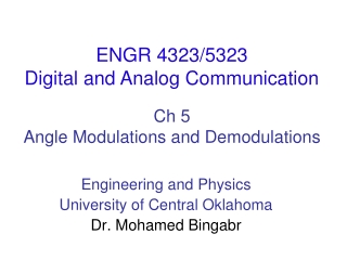
ENGR 4323/5323 Digital and Analog Communication. Ch 5 Angle Modulations and Demodulations. Engineering and Physics University of Central Oklahoma Dr. Mohamed Bingabr. Chapter Outline. Nonlinear Modulation Bandwidth of Angle Modulation Generating of FM Waves Demodulation of FM Signals

E N D
ENGR 4323/5323 Digital and Analog Communication Ch 5Angle Modulations and Demodulations Engineering and Physics University of Central Oklahoma Dr. Mohamed Bingabr
Chapter Outline • Nonlinear Modulation • Bandwidth of Angle Modulation • Generating of FM Waves • Demodulation of FM Signals • Effects of Nonlinear Distortion and Interference • Superheterodyne Analog AM/FM Receivers • FM Broadcasting System
Baseband Vs. Carrier Communications Angle Modulation: The generalized angle θ(t)of a sinusoidal signal is varied in proportion to the message signal m(t). Two types of Angle Modulation • Frequency Modulation: The frequency of the carrier signal is varied in proportion to the message signal. • Phase Modulation: The phase of the carrier signal is varied in proportion to the message signal. Instantaneous Frequency
Frequency and Phase Modulation Phase Modulation: Frequency Modulation: Power of an Angle-Modulated wave is constant and equal A2/2.
Example of FM and PM Modulation Sketch FM and PM waves for the modulating signal m(t). The constants kfand kp are 2πx105 and 10π, respectively, and the carrier frequency fc is 100 MHz.
Example of FM and PM Modulation Sketch FM and PM waves for the digital modulating signal m(t). The constants kfand kp are 2πx105 and π/2, respectively, and the carrier frequency fc is 100 MHz. Frequency Shift Keying (FSK) Phase Shift Keying (PSK) Note: for discontinuous signal kp should be small to restrict the phase change kpm(t)to the range (-π,π).
Bandwidth of Angle Modulated Waves where Expand using power series expansion The bandwidth of a(t), a2(t), an(t) are B, 2B, and nB Hz, respectively. From the above equation it seems the bandwidth of angle modulation is infinite but for practical reason most of the power reside at B Hz since higher terms have small power because of n!.
Narrowband PM and FM When kfa(t)<< 1 The above signal is Narrowband FM and its bandwidth is 2B Hz. Same steps can be carried out to find the Narrowband PM. Note: the above equation is similar to amplitude modulation but the waveform are different.
m(t) fc = 300 FM modulation kf = 120 kfa(t) = 6 NBFM (kfa(t)max <<1) fc = 300 PM modulation kp = 10 kpmp= 31.4NBPM (kpm(t)max << 1)
m(t) fc = 300 FM modulation kf = 10 kfa(t) = 0.5 NBFM (kfa(t)max <<1) fc = 300 PM modulation kp = 0.1 kpmp= 0.314NBPM (kpm(t)max << 1)
ts=1.e-4; kf= 10*pi; kp= 0.1*pi; fc = 300; t=-0.05:ts:0.05; Ta = 0.02; triangle = @(z)(1-abs(z)).*(z>=-1).*(z<1); m_sig= 1*(triangle((t+0.01)/Ta) - triangle((t-0.01)/Ta)); m_intg = ts*cumsum(m_sig); s_fm = cos(2*pi*fc*t + kf*m_intg); s_pm = cos(2*pi*fc*t + kp*m_sig); subplot(311); plot(t, m_sig) subplot(312); plot(t, s_fm) subplot(313); plot(t, s_pm) s_nbfm = cos(2*pi*fc*t) - kf*m_intg.*sin(2*pi*fc*t); s_nbpm = cos(2*pi*fc*t) - kp*m_sig.*sin(2*pi*fc*t); figure; subplot(311); plot(t, m_sig) subplot(312); plot(t,s_nbfm) subplot(313); plot(t, s_nbpm) figure; plot(t, m_intg) Code to demonstrate the effect of the condition for NBFM (kfa(t)max <<1) and NBPM (kpm(t)max << 1)
Wideband FM (WBFM) In many application FM signal is meaningful only if its frequency deviation is large enough, so kfa(t)<< 1 is not satisfied, and narrowband analysis is not valid. Fourier Transform + Hz Hz
Wideband FM (WBFM) Peak frequency deviation in hertz Hz A better estimate: Carson’s rule Hz is the deviation ratio Where When Δf >> B the modulation is WBFM and the bandwidth is BFM = 2 Δf When Δf << B the modulation is NBFM and the bandwidth is BFM = 2B
Wideband PM (WBPM) The instantaneous frequency Hz
Example Estimate BWFM and BWPM for the modulating signal m(t) for kf=2πx105and kp= 5π.Assume the essential bandwidth of the periodic m(t) as the frequency of its third harmonic. Repeat the problem if the amplitude of m(t) is doubled. Repeat the problem if the time expanded by a factor of 2: that is, if the period of m(t) is 0.4 msec.
Example An angle-modulated signal with carrier frequency ωc = 2 105 is described by the equation Find the power of the modulated signal. Find the frequency deviation Δf. Find the deviation ration . Find the phase deviation Δø. Estimate the bandwidth of . Read the Historical Note: Edwin H. Armstrong (page 270)
Generating FM Waves Two Methods: Indirect method using NBFM Generation Direct method NBFM Generation With the NBFM generation, the amplitude of the NBFM modulator will have some amplitude variation due to approximation.
Distortion with NBFM Generation Example 5.6:Discuss the nature of distortion inherent in the Armstrong indirect FM generator. Amplitude and frequency distortions.
NBFM Generation Bandpass Limiter
Generating FM Waves The output of the bandpass filter
Indirect Method of Armstrong NBFM is generated first and then converted to WBFM by using additional frequency multipliers. Example of frequency multiplier is a nonlinear device Devices of higher multiplier
Indirect Method of Armstrong For NBFM<< 1. For speech fmin = 50Hz, so if Δf = 25 then 25/50 = 0.5,
Example Design an Armstrong indirect FM modulator to generate an FM signal with carrier frequency 97.3 MHz and Δf = 10.24 kHz. A NBFM generator of fc1 = 20 kHz and Δf = 5 Hz is available. Only frequency doublers can be used as multipliers. Additionally, a local oscillator (LO) with adjustable frequency between 400 and 500 kHz is readily available for frequency mixing.
Direct Generation The frequency of a voltage-controlled oscillator (VCO) is controlled by the voltage m(t). Use an operational amplifier to build an oscillator with variable resonance frequency ωo. The resonance frequency can be varied by variable capacitor or inductor. The variable capacitor is controlled by m(t).
Direct Generation The maximum capacitance deviation is In practice Δf << fc
Demodulation of FM Signals A frequency-selective network with a transfer function of the form |H(f)|=2af + b over the FM band would yield an output proportional to the instantaneous frequency. Differentiator
Demodulation of FM Signals Differentiator
Practical Frequency Demodulators if The slope is linear over small band, so distortion occurs if the signal band is larger than the linear band. Zero-crossing detectors: First step is to use amplitude limiter and then the zero-crossing detector. Instantaneous frequency = the rate of zero crossing
Effect of Nonlinear Distortion and Interference Immunity of Angle Modulation to Nonlinearities Vulnerability of Amplitude Modulation to Nonlinearities
Interference Effect Angle Modulation is less vulnerable than AM to small-signal interference from adjacent channels. for I<<A The output of ideal phase and frequency demodulators are For PM Interference is inversely proportional to the carrier amplitude (capture effect). For FM
Preemphasis and Deemphasis in FM With white noise, the amplitude interference is constant for PM but increase with ω for FM. For audio signal the PSD is concentrated at low frequency below 2.1 kHz, so interference at high frequency will greatly deteriorate the quality of audio signal. Preemphasis Filter Deemphasis Filter Noise
Preemphasis and Deemphasis (PDE) in FM 30 kHz 2.1 kHz PreemphasisFilter DeemphasisFilter
Preemphasis and Deemphasis (PDE) in FM Where K is the gain and = ω2 /ω1 For 2f << ω1 For ω1 << 2f << ω2 PDE is used in many applications such as recording of audiotape and photograph recording, where PDE depends on the band.
FM Broadcasting Standard • Federal Communications Commission (FCC) specifications for FM communication • Frequency range = 88 to 108 MHz • Channel separations = 200 kHz, • Peak frequency deviation = 75 kHz • Transmitted signal should be received by monophonic and stereophonic receivers. Filter 150 KHz 75 KHz 88 89.8 90 90.2 108 MHz 200 KHz
Superheterodyne Analog AM/FM Receivers 90 desired signal 90.2 adjacent 111.4 image fc = 10.7 10.7 90 90.2 111.4 10.7 , 190.7 10.5 , 190.9 10.7, 212.1 90+10.7=100.7 fIF = 455KHz (AM radio); 10.7 MHz (FM); 38 MHz (TV) AM stations that are 2fIF apart are called image stations and both would appear simultaneously at the IF output. RF filter eliminates undesired image station, while IF filter eliminates undesired neighboring stations.
FM Broadcasting System Monophonic and Stereophonic Broadcasting System