Download
1 / 25
280 likes | 587 Views
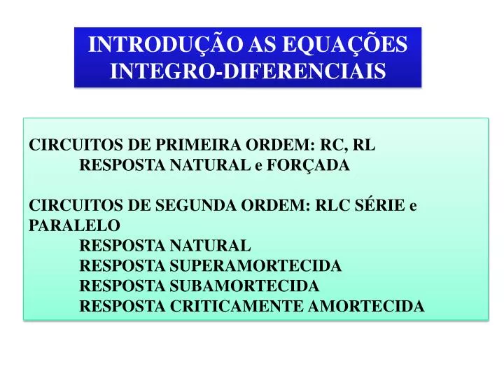
INTRODUÇÃO AS EQUAÇÕES INTEGRO-DIFERENCIAIS. CIRCUITOS DE PRIMEIRA ORDEM: RC, RL RESPOSTA NATURAL e FORÇADA CIRCUITOS DE SEGUNDA ORDEM: RLC SÉRIE e PARALELO RESPOSTA NATURAL RESPOSTA SUPERAMORTECIDA RESPOSTA SUBAMORTECIDA RESPOSTA CRITICAMENTE AMORTECIDA. Chave no lado direito

E N D
INTRODUÇÃO AS EQUAÇÕES INTEGRO-DIFERENCIAIS CIRCUITOS DE PRIMEIRA ORDEM: RC, RL RESPOSTA NATURAL e FORÇADA CIRCUITOS DE SEGUNDA ORDEM: RLC SÉRIE e PARALELO RESPOSTA NATURAL RESPOSTA SUPERAMORTECIDA RESPOSTA SUBAMORTECIDA RESPOSTA CRITICAMENTE AMORTECIDA
Chave no lado direito o capacitor se descarrega através da lâmpada. INTRODUÇÃO Com a chave no lado esquerdo o capacitor recebe carga da bateria.
RESPOSTA GERAL: CIRCUITO DE PRIMEIRA ORDEM IncluIindo a condição inicial no modelo do capacitor (tensão) ou no indutor (corrente): É denominada de constante de tempo e esta associada a resposta do circuito. Resolvendo a equação diferencial, usando o fator de integração, tem-se:
TEMPO CONSTANTE TRANSIENTE CIRCUITOS DE PRIMEIRA ORDEM COM FONTES CONSTANTES A forma da solução é: Qualquer variável do circuito é da forma: Somente os valores das constantes K1, K2 podem mudar
Tangente atinge o eixo x no valor da constante de tempo Descarrega de 0.632 do valor Inicial em uma constante de tempo Erro menor que 2% Transiente é zero a partir deste ponto EVOLUÇÃO DO TRANSIENTE E A INTERPRETAÇÃO DA CONSTANTE DE TEMPO VISÃO QUALITATIVA: MENOR CONSTANTE DE TEMPO MAIS RÁPIDO O TRANSITÓRIO DESAPARECE
CONSTANTE DE TEMPO O modelo: A solução pode ser escrita como: transiente Carga em um capacitor Para efeitos práticos, o capacitor é “carrregado” quando o transitório é insignificante.
EXAMPLE PASSO 1 CONSTANTE DE TEMPO PASSO 2 ANÁLISE DO ESTADO INICIAL NO ESTADO INICIAL A SOLUÇÃO É UMA CONSTANTE. A DERIVADA É ZERO. PASSO 3 USO DA CONDIÇÃO INICIAL
KVL PASSO 1 EXAMPLE PASSO 2 ESTADO INICIAL PASSO 3 CONDIÇÃO INICIAL
PROBLEMA PASSO 1 PASSO 2 PASSO 3
PASSO 1 PASSO 2 PASSO 3 INITIAL CONDITIONS É MAIS SIMPLES DETERMINAR ATRAVÉS DO MODELO DE TENSÃO
PASSO 1 PASSO 2 PASSO 3 EXEMPLO CONDIÇÃO INICIAL. CIRCUITO NO ESTADO INICIAL t<0
CIRCUITO NO ESTADO INICIAL EXEMPLO PASSO 3 PASSO 1 PASSO 2 CONDIÇÃO INICIAL CORRENTE NO INDUTOR PARA t<0
CIRCUITOS DE SEGUNDA ORDEM EQUAÇÃO BÁSICA Malha simples: Uso KVL Simples Nó: Uso KCL Diferenciando
MODEL O PARA RLC PARALELO MODELO PARA RLC SÉRIE EXEMPLO
A RESPOSTA DA EQUAÇÃO SE A FUNÇÃO FORÇADA É UMA CONSTANTE
EXEMPLO A EQUAÇÃO HOMOGÊNEA COEFICIENTE DA SEGUNDA DERIVADA RAZÃO DE DECAIMENTO, FREQ. NATURAL
(modes of the system) ANALISE DA EQUAÇÃO HOMOGÊNEA
DETERMINAR A FORMA DA SOLUÇÃO GERAL EXEMPLO Raizes complexas conjugadas Raizes reais e iguais SUBAMORTECIDO CRITICAMENTE AMORTECIDO
PROBLEMA Classificar a resposta para um dado valor de C EQUAÇÃO HOMOGÊNEA C=0.5 subamortecido C=1.0 criticamente amortecido C=2.0 superamortecido
To determine the constants we need EXEMPLO PASSO 1 MODELO ANALIZAR CIRCUITO t=0+ PASSO 2 PASSO 3 RAIZES PASSO 4 FORMA DA SOLUÇÃO PASSO 5: OBTER AS CONSTANTES
USO DO MATLAB PARA VISUALIZAR A RESPOSTA %script6p7.m %plots the response in Example 6.7 %v(t)=2exp(-2t)+2exp(-0.5t); t>0 t=linspace(0,20,1000); v=2*exp(-2*t)+2*exp(-0.5*t); plot(t,v,'mo'), grid, xlabel('time(sec)'), ylabel('V(Volts)') title('RESPONSE OF OVERDAMPED PARALLEL RLC CIRCUIT') SUPERAMORTECIDO
EXAMPLO model Form:
USO DO MATLAB PARA VISUALIZAR A RESPOSTA %script6p8.m %displays the function i(t)=exp(-3t)(4cos(4t)-2sin(4t)) % and the function vc(t)=exp(-3t)(-4cos(4t)+22sin(4t)) % use a simle algorithm to estimate display time tau=1/3; tend=10*tau; t=linspace(0,tend,350); it=exp(-3*t).*(4*cos(4*t)-2*sin(4*t)); vc=exp(-3*t).*(-4*cos(4*t)+22*sin(4*t)); plot(t,it,'ro',t,vc,'bd'),grid,xlabel('Time(s)'),ylabel('Voltage/Current') title('CURRENT AND CAPACITOR VOLTAGE') legend('CURRENT(A)','CAPACITOR VOLTAGE(V)') SUBAMORTECIDO
EXEMPL0 KVL KCL
Second Order USO DO MATLAB PARA VISUALIZAR A RESPOSTA %script6p9.m %displays the function v(t)=exp(-3t)(1+6t) tau=1/3; tend=ceil(10*tau); t=linspace(0,tend,400); vt=exp(-3*t).*(1+6*t); plot(t,vt,'rx'),grid, xlabel('Time(s)'), ylabel('Voltage(V)') title('CAPACITOR VOLTAGE') CRITICAMENTE AMORTECIDO