Download
1 / 30
300 likes | 400 Views
Learn about geospatial data aggregation and viewing with BI and Data Warehousing approaches, multi-level aggregation of point and linear data, data compilation workflows, and increasing data value. Explore how data aggregation supports decision-making, using pivot tables for data summarization and drilldown. Delve into a case study on Illinois, essential steps for handling point data, designing base tables, loading data, and building rollups. Discover how to use SQL for aggregation and rollup hierarchies. Understand ArcMap presentation requirements and drilldown processes.

E N D
GIS Rollup and Drilldown:Geospatial BI and Data Aggregation Brian Hebert ScribeKey, LLC May, 2011 www.scribekey.com
Presentation Overview • Look at geospatial data compilation and viewing using Business Intelligence (BI) and Data Warehousing approaches. • Show multi-level data aggregation of point and linear data using hierarchical polygon sets. • Review details of data compilation and presentation workflow. • GOAL: Help you get more value out of your data. • This presentation is part of a series looking at the application of BI and Data Warehousing in a geospatial context. • Related presentations and supporting materials can be found at www.scribekey.com, including Data Profiling, Meta-Layers, Data Dictionary Generation, Data Quality, etc. www.scribekey.com
The Value of Data Aggregation in Decision Support • Data aggregation provides a key component of decision support information systems, AKA, Business Intelligence (BI). • Provides a smaller, faster, high level summary and simplification of large volumes of data. • Helps decision makers focus in on what’s important. • Created using standard RDBMS SQL aggregation constructs, SUM, COUNT, and GROUP BY and OLAP technology. AGGREGATE BASE DATA www.scribekey.com
The Pivot Table • Provides easy-to-use summary and drilldown/rollup views of data. • Very flexible for defining rows, columns, and filters • Available with MS Excel, Access, and in OLAP environments • Used extensively in Business Intelligence and Data Warehousing HOW CAN WE MAKE A PIVOT MAP, TO GET THE SAME CAPABILITY WITH GIS? www.scribekey.com
GOAL: The Pivot Map Increasingly detailed views COUNTY TOWN Applying Pivot Table like view and Drilldown/Rollup with hierarchical geography units CENSUS TRACT www.scribekey.com 5
Example Case Study: ILLINOIS • Sample CENSUS data for the State of Illinois. • Using point and linear data. • POIs, FOIs, Widgets; think of this as your data. • Compile linear Railroad feature lengths and display results using shaded polygons. • Utilities, Infrastructure, Disease Surveillance, Crime, Transportation, Data Holdings, etc. www.scribekey.com
3 Essential Requirements and Steps With point data, assume we have GEOCODED base info, e.g., sales, crime, disease, critical infrastructure, demographics • SPATIAL JOIN: Assign points, lines to hierarchical sets of geographic units, as polygons, e.g., country, region, state, marketing areas, legislative disticts, county, city/town, ZipCode, census tract/block-group, block, etc. • AGGREGATION: Generate rollup views/tables using SQL SUM, COUNT, GROUP BY, as views and tables. • PRESENTATION: Provide tools for presenting the rollups, e.g., reports, drilldown/pivot tables, drilldown maps, etc. www.scribekey.com
Designing the Base Table • For FOIs, create table with types, numeric quantities, time, and hierarchical geography assignments IN OLAP TERMINOLOGY, DATA GROUPING CATEGORIES ARE CALLED DIMENSIONS, NUMERICAL QUANTITIES ARE CALLED MEASURES www.scribekey.com
Loading the Base Table • Can use SPATIAL JOIN multiple times, from ArcToolbox, creates new datasets • For large number of geographies, write custom application with ArcObjects, for each point, cycle through a number of geographies doing a Point-In-Polygon operation • Economies to be gained with nested, hierarchical IDs, e.g., Census www.scribekey.com
Base Table Contents WITH BASE TABLE IN PLACE, CAN START TO BUILD AGGREGATE ROLLUPS WITH SQL www.scribekey.com
Building the Rollups with SQL • For numeric fields, we use aggregate functions, SUM(), MIN(), MAX(), AVG(), STD(). • Always include COUNT(*). • Use of GROUP BY to aggregate by Type, Geography, Time, etc. • There are lots of possible permuations. • This is what PIVOT TABLE or CUBE does, creates all possible views using the measures and dimensions. www.scribekey.com
Building the Rollups with SQL (cont.) SELECT COUNTYID, COUNTY, TYPE, COUNT(*), SUM(AMT) [INTO POI_COUNTY] FROM POI_BASE GROUP BY COUNTYID, COUNTY, TYPE Depending on dataset size, use VIEWS or create actual TABLES. www.scribekey.com
Rollup Hierarchy ROLLUPS PROVIDE COUNTY, TOWN, CENSUS TRACT HIERARCHY AND AGGREGATES www.scribekey.com
ArcMap Presentation Requirements • Add base polygon layers • Add rollup tables • Link through Joins and Relates • Set symbolization, classification, color shading www.scribekey.com
Anatomy of Drilldown • Select high-level parent feature, view attributes • View related child records, RELATE SELECT • Drill down to view next level geography • Turn layers on/off • Zoom to selection • Lots of individual operations, mouse clicks, can be consolidated using ArcObjects www.scribekey.com
Table Driven Presentation Load from DB C# Code Facsimile: string[,] LayerFamilyTree = new string[3, 4] { { "Counties", "tl_2009_17_county00", "CNTYIDFP00", "NA"}, { "Towns", "tl_2009_17_cousub00", "COSBIDFP00", "tl_2009_17_county00"}, { "Tracts", "tl_2009_17_tract00", "CMTIDFP00", "tl_2009_17_cousub00"} }; ArcObjects Drilldown and Rollup presentation tools can be driven by tabular data which captures the hierarchical relationship between parent and child feature layers. This is a form of metadata typically found in OLAP environments, and is the same information used to capture the relationships with Point-In-Polygon routine. www.scribekey.com
Additional Presentation Options Showing 2 hierarchical levels at the same time with Transparency Showing only the features in the current family tree with Query Filter www.scribekey.com
Other Considerations • Using partitioned data • Use of more advanced formulas in SQL • Use of linear data lengths • Use of area data measurements • Non-hierarchical geography • Metadata: Meta-Layers www.scribekey.com
Partitioned Data • For a variety of reasons, data is often partitioned. • Example: US Census data, by State, then County • This data can be used, as-is, without needing to merge it all into one set of large layers. • Using partitioned data can increase performance considerably. • Consequences for 3 main GeoRollup activities: • SPATIAL JOIN: Perform a 2-pass operation, e.g., find the town first, then the parcel. • AGGREGATION: More granular operation with separate tables, but these can be merged using SQL UNION, etc. • PRESENTATION: More granular file and layer management for zoom-to-extents, layers on/off, etc. www.scribekey.com
More Advanced Formulas • When you want to see more than simple count(*) or sum() • Case Study: EPIGIS Disease Surveillance • Cancer cases by gender, age, cancer type, etc. used with population data. • Can be expressed in SQL and aggregated by geography. • Case count aggregation used as numerator over population to present incidence by Town, and drilldown to Census Tract. SELECT Gender, Age, CancerType, Town, CensusTract, Count(*) AS Cases, Count(*)/Sum(Pop) As Rate FROM CancerData GROUP BY Gender, Age, CancerType, Town, CensusTract www.scribekey.com
Linear Data: Length Calculation • Example use case: Need to see length in miles of Railroad related to population. • May need to break lines at polygon boundaries. • Lon/Lat data needs to be projected to use Geometry Calculator or can use great circle distance. • Aggregate data and FEET->MILES conversion using SQL: • SELECT ROUND(SUM(LEN_FT)/5280, 2) as LEN_MI www.scribekey.com
Rail Length In Miles By Town in Cook Country • Extracted only RAILFLG=‘Y’ from Cook Country Streets • Projected to ILLINOIS State Plane Feet • Performed Calculate Geometry Length • Performed SPATIAL JOIN with Town layer • Used SQL to perform aggregation: • SELECT • NAME00 AS Town, • Round(Sum(LEN_FT)/5280,2) AS LEN_MI • INTO RRLenByTown • FROM CookCoRR • GROUP BY • NAME00 • Added new field to town layer and updated • Added layer to ArcMap, set Symbology to 3 classes using RR_LEN_MI www.scribekey.com
Area Measurements and Non-Hierarchical Sets • Like points and linear features, areas can be aggregated by size, type, etc. • Relationship between polygon layers is not always hierarchical, example: ZIP Codes and Towns. Can use intersection and hybrid layer. • Also, phenomena is not evenly distributed over a polygon area. • Aggregation transfer approaches can use street network or population polygons as proxy. • Shared boundary features inclusion issue. www.scribekey.com
Viewing Metadata: Meta-Layers • Different kinds of metadata: • Database metadata as name, data type, length of fields • FGDC metadata as info about both layer, e.g., feature geometry type, projection, and individual attributes, domains • Aggregation metadata as summary count(*), sum(), etc. values • Metadata can be managed and viewed as GIS layers, using polygons to represent coverage areas, and metadata elements loaded into RDBMS tables. www.scribekey.com
1st Step: Data Profile and FGDC Metadata in DB • Data profiling captures structure and contents information from data, e.g., record counts, attribute counts, attribute names, data types, percent complete, etc. • Import FGDC Entity, Attribute, and Domain values and definitions into tabular database tables. www.scribekey.com
Add and Join/Relate Metadata Tables in ArcMap: Meta-Layers • Integrate data profiling and FGDC metadata in RDBMS • Data quality, percent complete, etc. • Add as table to ArcMap • Metadata available like other tabular data in ArcGIS • N->1 Attribute->Entity • HTML Data Dictionary www.scribekey.com
OLAP 101 • Read-only database, not normalized • Measures and Dimensions • Star and Snowflake schemas • MDX, XMLA Cube Query Languages • Metadata Repository • There is no middle tier, pure query language behind the interfaces METADATA REPOSITORY www.scribekey.com
Why is there a GIS/BI Technology Gap? • GIS has evolved independently of mainstream RDBMS OLTP/OLAP because of the variable length geometry and spatial operations. • GIS schemas and applications have focused on read-write production databases, not read-only decision support databases. • GIS standards bodies have focused on XML as opposed to RDBMS schemas for production databases and metadata, again, not decision support databases. • BI tools and techniques typically don’t handle geometric operations, e.g., spatial join, dissolve, etc. • There are some fledging solutions, SAS/ESRI Bridge, MS SQL Server RS Map Control, QlikView/Map integration. • One ultimate goal would be to link and drive a GIS display engine from an OLAP Cube. www.scribekey.com
Recap and Take Aways • Applying OLAP data compilation and viewing techniques can provide very rich data views and powerful decision support. • Try using pivot tables in MS Excel or Access, get familiar with concepts, reproduce similar views in ArcMap. • Focus on creation of base table, then rollup with SQL COUNT(*), SUM(), GROUP BY. • Learn about and explore OLAP, BI, Data Warehousing. • Learn about data profiling and put FGDC metadata into data tables that can be viewed in ArcMap www.scribekey.com
Thank YouQuestions and Answers www.scribekey.com