Linear Least Square s Problem

1. Linear Least Squares Problem • Over-determined systems • Minimization problem: Least squares norm • Normal Equations • Singular Value Decomposition Lecture 4

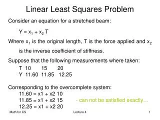
2. Linear Least Squares: Example Consider an equation for a stretched beam: Y = x1 + x2 T Where x1 is the original length, T is the force applied and x2 is the inverse coefficient of stiffness. Suppose that the following measurements where taken: T 10 15 20 Y 11.60 11.85 12.25 Corresponding to the overcomplete system: 11.60 = x1 + x2 10 11.85 = x1 + x2 15 - can not be satisfied exactly… 12.25 = x1 + x2 20 Lecture 4

3. Linear Least Squares: Definition Problem: Given A(m x n), m≥n, b(m x 1) find x(n x 1) to minimize ||Ax-b||2. • If m > n, we have more equations than the number ofunknowns, there is generally no x satisfying Ax=b exactly. • This is an overcomplete system. Lecture 4

4. Solution Approaches There are three different algorithms for computing the least square minimum. • Normal Equations (Cheap,less Accurate). • QR decomposition. • SVD(expensive,more reliable). The first algorithm in the fastest and the least accurateamong the three. On the other hand SVD is the slowest and most accurate. Lecture 4

5. Normal Equations 1 Minimize the squared Euclidean norm of the residual vector: To minimize we take the derivative with respect to x and set it to zero: Which reduces to an (n x n) linear system commonly known as NORMAL EQUATIONS: Lecture 4

6. x b A Normal Equations 2 11.60 = x1 + x2 10 11.85 = x1 + x2 15 12.25 = x1 + x2 20 min||Ax-b||2 Lecture 4

7. Normal Equations 3 We must solve the system For the following values (ATA)-1ATis called a Pseudo-inverse Lecture 4

8. QR factorization 1 • A matrix Q is said to be orthogonal if its columns are orthonormal, i.e. QT·Q=I. • Orthogonal transformations preserve the Euclidean norm since • Orthogonal matrices can transform vectors in various ways, such as rotation or reflections but they do not change the Euclidean length of the vector. Hence, they preserve the solution to a linear least squares problem. Lecture 4

9. QR factorization 2 Any matrix A(m·n) can be represented as A = Q·R ,where Q(m·n) is orthonormal and R(n·n) is upper triangular: Lecture 4

10. QR factorization 2 • Given A , let its QR decomposition be given as A=Q·R, where Q is an (m x n) orthonormal matrix and R is upper triangular. • QR factorization transform the linear least square problem into a triangular least squares. Q·R·x = b R·x = QT·b x=R-1·QT·b Matlab Code: Lecture 4

11. Singular Value Decomposition • Normal equations and QR decomposition only work for fully-ranked matrices (i.e. rank( A) = n). If A is rank-deficient, that there are infinite number of solutions to the least squares problems and we can use algorithms based on SVD's. • Given the SVD: U(m x m) , V(n x n) are orthogonal Σ is an (m x n) diagonal matrix (singular values of A) The minimal solution corresponds to: Lecture 4

12. Singular Value Decomposition Matlab Code: Lecture 4

13. Linear algebra review - SVD Lecture 4

14. Approximation by a low-rank matrix Lecture 4

15. σ·v1 v1 σ·v2 v2 Geometric Interpretation of the SVD The image of the unit sphere under any mxn matrix is a hyperellipse Lecture 4

16. S AS v1 σ·u1 σ·u2 v2 Left and Right singular vectors We can define the properties of A in terms of the shape of AS Singular values of A are the lengths of principal axes of AS, usually written in non-increasing order σ1 ≥ σ2 ≥ … ≥ σn n left singular vectorsof A are the unit vectors {u1,…, un}, oriented in the directions of the principal semiaxes of AS numbered in correspondance with {σi} n right singular vectorsof A are the unit vectors {v1,…, vn}, of S, which are the preimages of the principal semiaxes of AS: Avi= σiui Lecture 4

17. Singular Value Decomposition Avi= σiui, 1 ≤ i ≤n - Singular Value decomposition Matrices U,V are orthogonal and Σ is diagonal Lecture 4

18. Matrices in the Diagonal Form Every matrix is diagonal in appropriate basis: Any vector b(m,1) can be expanded in the basis of left singular vectors of A {ui}; Any vector x(n,1) can be expanded in the basis of right singular vectors of A {vi}; Their coordinates in these new expansions are: Then the relation b=Ax can be expressed in terms of b’ and x’: Lecture 4

19. Rank of A Let p=min{m,n}, let r≤p denote the number of nonzero singlular values of A, Then: The rank of A equals to r, the number of nonzero singular values Proof: The rank of a diagonal matrix equals to the number of its nonzero entries, and in the decomposition A=UΣV* ,U and V are of full rank Lecture 4

20. Determinant of A For A(m,m), Proof: The determinant of a product of square matrices is the product of their determinants. The determinant of a Unitary matrix is 1 in absolute value, since: U*U=I. Therefore, Lecture 4

21. A in terms of singular vectors For A(m,n), can be written as a sum of r rank-one matrices: (1) Proof: If we write Σ as a sum of Σi, where Σi=diag(0,..,σi,..0), then (1) Follows from (2) Lecture 4

22. Norm of the matrix The L2 norm of the vector is defined as: (1) The L2 norm of the matrix is defined as: Therefore ,where λi are the eigenvalues Lecture 4

23. Matrix Approximation in SVD basis For any ν with 0 ≤ ν ≤r, define (1) If ν=p=min{m,n}, define σv+1=0. Then Lecture 4