Download
1 / 53
530 likes | 837 Views
Einstein and Brownian Motion or How I spent My Spring Break ( not in Fort Lauderdale ). C. Jui Undergraduate Seminar March 25, 2004. I will make available this presentation at http://www.physics.utah.edu/~jui/brownian. Acknowledgments. My thanks to:

E N D
Einstein and Brownian MotionorHow I spent My Spring Break(not in Fort Lauderdale) C. Jui Undergraduate Seminar March 25, 2004 I will make available this presentation at http://www.physics.utah.edu/~jui/brownian
Acknowledgments My thanks to: Sid Rudolph, the director of the ACCESS program, which is designed to integrate women into science, mathematics, and engineering careers. Gernot Laicher, the director of Elementary Laboratory, who also prepared the micro-sphere suspension and took the video sequence of Brownian motion.
Acknowledgments (continued) Also thanks to: Lynn Monroe and Dr. Wilson of the Ken-A-vision Company who loaned us the T-1252 microscope which we used to make the measurement of Avogadro’s Number from Brownian Motion
Outline • What is Brownian Motion • The phenomenon 1827-1000 • Einstein’s paper of 1905 • Langevin’s Complete Derivation • My Science Fair Project (How I spent my Spring Break) • Epilogue
What is Brownian Motion? • #1 answer from Google (Dept. of Statistics) http://galton.uchicago.edu/~lalley/Courses/313/WienerProcess.pdf
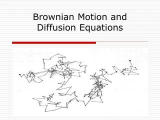
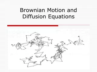
Other answers From computer Science at Worcester Polytechnic Inst. http://davis.wpi.edu/~matt/courses/fractals/brownian.htmlBrownian Motion is a line that will jump up and down a random amount and simular to the "How Long is the Coast of Britain?" problem as you zoom in on the function you will discover similar patterns to the larger function. The two images above are examples of Brownian Motion. The first being a function over time. Where as t increases the function jumps up or down a varying degree. The second is the result of applying Brownian Motion to the xy-plane. You simply replace the values in random line that moves around the page.
Electrical Engineering • A less commonly referred to 'color' of noise is 'brown noise'. This is supposed simulate Brownian motion a kind of random motion that shifts in steady increments. 'Brown noise' decreases in power by 6 dB per octave.
The source of Confusion • There are two meanings of the term Brownian motion: • the physical phenomenon that minute particles immersed/suspended in a fluid will experience a random movement • the mathematical models used to describe the physical phenomenon. • Quite frequently people fail to make this distinction
Brownian Motion: Discovery • Discovered by Scottish botanist Robert Brown in 1827 while studying pollens of Clarkia (primrose family) under his microscope
Robert Brown • Robert Brown’s main claim to fame is his discovery of the cell nucleus when looking at cells from orchids under his microscope 20 orchid epidermal cells showing nuclei (and 3 stomata) seen under Brown’s original microscope preserved by the Linnean Society London
Brown’s Microscope • And Brownian motion of milk globules in water seen under Robert Brown’s microscope
Brown’s Observations • At first Brown suspected that he might have been seeing locomotion of pollen grains (I.e. they move because they are alive) • Brown then observed the same random motion for inorganic particles…thereby showing that the motion is physical in origin and not biological. • Word of caution for the Mars Exploration program: Lesson to be learned here from Brown’s careful experimentation.
1827-1900 • Desaulx (1877): • "In my way of thinking the phenomenon is a result of thermal molecular motion (of the particles) in the liquid environment” • G.L. Gouy (1889): • observed that the "Brownian" movement appeared more rapid for smaller particles
F. M. Exner (1900) • F.M. Exner (1900) • First to make quantitative studies of the dependence of Brownian motion on particle size and temperature • Confirmed Gouy’s observation of increased motion for smaller particles • Also observed increased motion at elevated temperatures
Louis Bachelier (1870-1946) • Ph.D Thesis(1900): "Théorie de la Spéculation" Annales de l'Ecole normale superiure • Inspired by Brownian motion he introduced the idea of “random-walk” to model the price of what is now called a barrier option (an option which depends on whether the share price crosses a barrier).
Louis Bachelier (continued) • The “random-walk” model is formally known as “Wiener (stochastic) process” and often referred to as “Brownian Motion” • This work foreshadowed the famous 1973 paper: Black F and Scholes M (1973) “The Pricing of Options and Corporate Liabilities” Journal of Political Economy81 637-59 • Bachelier is acknowledged (after 1960) as the inventor of Mathematical Finance (and specifically of Option Pricing Theory)
Fischer Black died in 1995 Myron Scholes shared the 1997 Nobel Prize in economics with Robert Merton New Method for Calculating the prize ofderivatives Black and Scholes
Albert Einstein • Worked out a quantitative description of Brownian motion based on the Molecular-Kinetic Theory of Heat • Published as the third of 3 famous three 1905 papers • Awarded the Nobel Prize in 1921 in part for this.
Einstein’s 1905 papers • On a Heuristic Point of View on the Creation and Conversion of Light (Photo-Electric Effect) http://lorentz.phl.jhu.edu/AnnusMirabilis/AeReserveArticles/eins_lq.pdf • On the Electrodynamics of Moving Bodies (Theory of Special Relativity) http://www.fourmilab.ch/etexts/einstein/specrel/www/ • Investigation on the Theory of the Brownian Movement http://lorentz.phl.jhu.edu/AnnusMirabilis/AeReserveArticles/eins_brownian.pdf
Historical Context • Einstein’s analysis of Brownian Motion and the subsequent experimental verification by Jean Perrin provided 1st “smoking gun” evidence for the Molecular-Kinetic Theory of Heat • Kinetic Theory is highly controversial around 1900…scene of epic battles between its proponents and its detractors
Molecular-Kinetic Theory • All matter are made of molecules (or atoms) • Gases are made of freely moving molecules • U (internal energy) = mechanical energy of the individual molecules • Average internal energy of any system: U=nkT/2, n = no. of degrees of freedom • Boltzmann: Entropy S=klogW where W=no. of microscopic states corresponding to a given macroscopic state
Ludwig Boltzmann (1844-1906) Committed suicide in 1906. Some think this was because of the vicious attacks he received from the Scientific Establishment of the Day for his advocacy of Kinetic Theory Boltzmann’s tombstone in Vienna
Einstein’s Paper • In hindsight Einstein’s paper of 1905 on Brownian Motion takes a more circuitous route than necessary. • He opted for physical arguments instead of mathematical solutions • I will give you the highlights of the paper rather than the full derivations • We will come back to a full but shorter derivation of Paul Langevin (1908)
Section 1: Osmotic Pressure • Einstein reviews the Law of Osmotic Pressure discovered by J. van’t Hoff who won the Nobel Prize in Chemistry for this in 1901 In a dilute solution: p= osmotic pressure n = solute concentration N = Avogadro’s number R = gas constant T = absolute temperature
Section 1 (continued) • Einstein also argues that from the point of view of the Kinetic Theory the Law of Osmotic Pressure should apply equally to suspension of small particles
Section 2 • Einstein derives the Law of Osmotic Pressure as a natural consequence of Statistical Mechanics • The law minimizes the Helmholtz Free Energy with entropy calculated following Boltzmann’s prescription
Section 3: Diffusion • Using Statistical Mechanics (minimizing free energy) Einstein shows that a particle (in suspension) in a concentration gradient (in x) will experience a force K given (in magnitude) by • This force will start a flow of particles against the gradient.
Diffusion (continued) • Assuming a steady state flow (in a constant gradient and in a viscous medium) the particles will reach terminal velocity of Here p = 3.1415.. h = viscosity of fluid medium a = radius of spherical particles executing Stokes flow and experiencing a resistive force of
Diffusion (continued) • The resulting flux of particles is then given by Resulting in a definite prediction for the diffusion constant D given by This result a prediction of Kinetic Theory can be checked experimentally in Brownian Motion!
Section 4: Random Walk • Einstein then analyzes the Brownian Motion of particles suspended in water as a 1-d random walk process. • Unaware of the work of Bachelier his version of random walk was very elementary • He was able to show with his own analysis that this random walk problem is identical to the 1-d diffusion problem
Random Walk (continued) • The 1-d diffusion equation is • This equation has the Green’s Function (integral kernel) given by • Which is then the expected concentration of particles as a function of time where all started from the origin.
Section 5: Average x2 • Taking the initial position of each particle to be its origin then the average x2 is then given by • Einstein finishes the paper by suggesting that this diffusion constant D can be measured by following the motion of small spheres under a microscope • From the diffusion constant and the known quantities Rh and a one can determine Avogadro’s number N
Jean Perrin (1870-1942) • Using ultra-microscope Jean Perrin began quantitative studies of Brownian motion in 1908 • Experimentally verified Einstein’s equation for Brownian Motion • Measured Avogadro’s number to be N = 6.5-6.9x10²³ • From related work he was the first to estimated the size of water molecules • Awarded Nobel Prize in 1926
Paul Langevin (1872-1946) • Most known for: • Developed the statistical mechanics treatment of paramagnetism • work on neutron moderation contributing to the success to the first nuclear reactor • The Langevin Equation and the techniques for solving such problems is widely used in econometrics
Langevin Equation • In 1908 Paul Langevin developed a more direct derivation based on a stochastic (differential) equation of motion. We start with Newton’s 2nd Law (Langevin Equation): h = viscosity of water Fext is a “random” force on the particle
Scalar product by r • We now take the dot (scalar product) of the equation of motion by r : • Next we re-express the above equation in terms of r2instead.
Ensemble Average • The equation of motion now becomes: • Rearranging the equation and denoting ||dr/dt||2=V2 • Next we take the average over a large number of particles (“ensemble average” denoted by ) and using u r2
The Physics!!! 0 • The last term on the right vanishes because Fext is a “random” force not correlated with the position of the particle. • By Equi-partition Theorem we have ½MV2 = nkT/2 (a constant!) where n is the number of spatial dimensions involved and k is again the Boltzmann Constant. PHYSICS!!!
Solving the Differential Equation A 2nd order linear inhomogenous ODE: where and • Using MAPLE to solve this :
Initial Conditions • r2 = 0 at t = 0 • Assuming initial position of each particle to be its origin. • dr2/dt= 0 at t = 0 • At very small t (I.e. before any subsequent collisions) we have ri2 = (Vit)2 where Vi is the velocity the ith particle inherited from a previous collision. r2 = V2 t2 dr2/dt |t=0 = 0
Applying Initial Conditions • We arrive at the solution
Langevin: t << t case • Expanding the exponential in Taylor series to 2nd order in t. Note 0th and 1st order terms cancel with the two other terms.
Langevin: t >> t case • Taking the other extreme which is the case of interest • Which is the same as Einstein’s result but with an extra factor of n (Note Einstein’s derivations were for a 1-d problem)
My Science Fair Project(How I Spent my Spring Break) • We are setting up a Brownian motion experiment for UGS 1430 (ACCESS summer program) and for PHYCS 2019/2029 • Will use inexpensive Digital microscopes with a 100X objective • Use 1 mm diameter (3% uniformity) polystyrene • Did a “fun” run using an even cheaper digital scope with a 40X objective
The Tool • Used a Ken-A-Vision T-1252 Digital Microscope loaned to us by the company • Up to 40X objectve • USB interface for video capture
Data Analysis t(s) x y 0 238 414 10 246 402 20 247 396 30 246 397 40 250 405 50 238 403 60 228 414 70 227 400 80 225 397 90 241 409 100 234 408 110 236 408 120 238 410 • Followed 14 particles for 80 seconds • digitized x and y position every 10 seconds using Free package “DataPoint” http://www.stchas.edu/faculty/gcarlson/physics/datapoint.htm • Raw data for particle #9 shown to the right (x, y coordinates in pixels)
Data Analysis (continued) • Some “bulk flow” was observed: x and y were non-zero and changed steadily with time. For pure Brownian motion these should be constant AND zero • To account for the flow we used sx2=x2-x2 and sy2= y2-y2 instead of just x2 and y2 in the analysis