Teachable Unit: Brownian Motion
Teachable Unit: Brownian Motion. Created by: Claudia De Grandi and Katherine Zodrow May 2013. claudia.degrandi@yale.edu katherine.zodrow@yale.edu. Unit Summary. This unit contains materials for 2 or 3 class periods. Parts of this unit can stand alone. Teaching Materials Include

Teachable Unit: Brownian Motion
E N D
Presentation Transcript
Teachable Unit:Brownian Motion Created by: Claudia De Grandi and Katherine Zodrow May 2013 claudia.degrandi@yale.edu katherine.zodrow@yale.edu
Unit Summary • This unit contains materials for 2 or 3 class periods. Parts of this unit can stand alone. • Teaching Materials Include • Powerpoint slides detailing unit • Powerpoint slides to be used in the classroom • 2 Matlab modules (for beginners) to help explain Brownian motion • In class quiz/questions • Homework
Part 1 (75 min) • Introduce learning goals • Perform a 1D random walk as a class • History of Brownian motion (lecture) • Reflection and discussion
Part 2 (75 min) • Present and discuss the solutions to the homework (from Part 1) • Computer lab group activity with Matlab (Module I) • Students follow instructions on handout to simulate and analyze 1D random walks • Students hand in a final lab report • Students are given final answer key sheet • TAs and Instructor available for in-class help
Part 3 (75 min) • Introduction to data analysis: How do researchers use Brownian motion? • Computer lab group activity with Matlab on 2D random walks (Module II) • Final question: Estimate the radius of an atom • Discuss solution of the question • Reflection, final comments on initial learning goals.
Assessment • Initial reflection on learning goals questions (see slide 9) • Initial multiple choice quiz about binomial distribution (see slide 11) • Homework (end of Part 1) on diffusion in different viscosities • 2 Matlab Modules, to be turned in as a short lab report • In-class final problem questions about the size of an atom • Final homework/report: revised and detailed answers to learning goals questions
Materials needed • coin to flip for each student • a relatively spacious room to implement the random walk activity or a large white board and Post-it stickers • a computer and screen to project slides • Device for students to use Learning Catalytics (formative assessment questions and class random walk activity) • Computer with Matlab for each student group • Handout for students with a copy of the slides
Brownian motion, Atoms and Avogadro’s Number • How do we know atoms exist? • What is the size of an atom? • How would you observe an individual atom?
Brownian motion, Atoms and Avogadro’s Number • How do we know atoms exist? • What is the size of an atom? • How would you observe an individual atom? Suggestion: make a ‘diary’ to keep track of your learning process At the end of the 3 lectures your homework will be to summarize what you have learned and give your best answers to those questions.
Today in class, we will • Review the binomial distribution: quiz • Perform a 1D random walk as a class and extract our diffusion coefficient • Review the history of Brownian motion: • R. Brown(1827): botanist observing motion of pollen grains • Einstein’s theory and connection to Avogadro’s number (1905) • Perrin’s experiment (1908)
p = probability of one success average number of successes : variance : reminder probability of k successes in n trials Binomial Distribution
understand how the variance • depends on time Learning goals: • extract the diffusion coefficient D
understand how to extract the diffusion • coefficient from 2D images • relate the diffusion coefficient to the • Avogadro’s number Learning goal:
Pressure Temperature Ideal gas law Volume ideal gas constant
Pressure total number of molecules Temperature Boltzmann constant Ideal gas law Volume ideal gas constant # of moles In our case: water mole=as many molecules as in 12 grams of 12C mole= Avogadro’s number(NA) of molecules
Pressure total number of molecules Temperature Boltzmann constant historically Ideal gas law Volume ideal gas constant # of moles Einstein’s theory of Brownian motion! In our case: water mole=as many molecules as in 12 grams of 12C mole= Avogadro’s number(NA) of molecules
Einstein’s theory
Einstein’s theory
Einstein’s theory
Einstein’s theory Friction coefficient Diffusion coefficient
Einstein’s theory Radius of green particles viscosity Friction coefficient measurable! in Brownian motion Diffusion coefficient
Einstein’s theory time Radius of green particles viscosity Friction coefficient measurable! in Brownian motion Diffusion coefficient known quantities
Today’s Recap Diffusion coefficient of 1D random process Diffusion coeff. of 2D brownian particles Einstein’s theory Avogadro’s number!
Brownian motion, Atoms and Avogadro’s Number • How do we know atoms exist? • What is the size of an atom? • How would you observe an individual atom?
Homework • At 20 °C, the dynamics viscosity η of water is 10-3 Pa*s. Glycerol is 1Pa*s. We place particles in these two solutions, holding everything else constant. Give a quantitative relationship for the diffusion of these particles in these two solutions. • Sketch a plot that compares <x2>vs. time for particles in each of these solutions.
Today in class, we will • Review solutions to the homework • Use Matlab software to simulate and analyze in details 1D random walks • Work in groups of 2/3 people • Follow instruction on handout • Hand in a report by the end of the lecture
Today in class, we will • Use Matlab software to simulate and analyze 2D Brownian motion (like reproducing Perrin’s exp. images) • Work in groups as Module I, hand in final report • You will extract the Avogadro’s number from your data • Group problem: estimate the size of a molecule from Avogadro’s number • Final discussion on learning goals and final homework
Estimate of molecular radius Assume Avogadro’s number NA= 6 X10²³ NA is the total number of molecules in a mole Reminder Ideal gas law: Work in groups to find an estimate of the size of a molecule in a mole
Estimate of molecular radius volume of a mole at room Temp. (T=300) and 1 atm.(100kPa) estimate of particles radius
Brownian motion, Atoms and Avogadro’s Number • How do we know atoms exist? • What is the size of an atom? • How would you observe an individual atom? Final homework/report/reflection: write down your best answers, compare with your initial guess, discuss what are the most important things you have or have not learned during this teaching unit
Additional reading • Haw, M D. (2002) Colloidal suspensions, Brownian motion, molecular reality: a short history. J. Phys. Condens. Matter 14:7769. • Philip Nelson’s book: Biological physics: Energy, Information, Life (Chap. 4). • Random Walks in Biology, Howard Berg • Investigation on the theory of The Brownian Movement, Albert Einstein, Dover Publications (1956) (original Einstein’s paper on Brownian motion).