Chapter 3 Brownian Motion
Chapter 3 Brownian Motion. 3.2 Scaled random Walks. 3.2.1 Symmetric Random Walk. To construct a symmetric random walk, we toss a fair coin (p, the probability of H on e ach toss, and q, the probability of T on e ach toss). 3.2.1 Symmetric Random Walk. Define , k=1,2,….

Chapter 3 Brownian Motion
E N D
Presentation Transcript
Chapter 3 Brownian Motion 3.2 Scaled random Walks
3.2.1 Symmetric Random Walk • To construct a symmetric random walk, we toss a fair coin (p, the probability of H on each toss, and q, the probability of T on each toss)
3.2.1 Symmetric Random Walk • Define • , k=1,2,…..
3.2.2 Increments of the Symmetric Random Walk • A random walk has independent increments .If we choose nonnegative integers 0 = , the random variables are independent • Each is called incrementof the random walk
3.2.2 Increments of the Symmetric Random Walk • Each increment has expected value 0 and variance
3.2.3 Martingale Property for the Symmetric Random Walk • Choose nonnegative integers k < l , then
3.2.4 Quadratic Variation for the Symmetric Random Walk • The quadratic variation up to time k is defined to be • Note : .this is computed path-by-path and .by taking all the one-step increments along that path, squaring these increments, and then summing them
3.2.5 Scaled Symmetric Random Walk • To approximate a Brownian motion • Speed up time of a symmetric random walk • Scale down the step size of a symmetric random walk • Define the Scaled Symmetric Random Walk • If nt is not an integer, we define by linear interpolation • is a Brownian motion as
3.2.5 Scaled Symmetric Random Walk • Consider • n=100 , t=4
3.2.5 Scaled Symmetric Random Walk • The scaled random walk has independent increments • If 0 = are such that each is an integer, then are independent • If are such that ns and nt are integers, then
3.2.5 Scaled Symmetric Random Walk • Scaled Symmetric Random Walk is Martingale • Let be given and s , t are chosen so that ns and nt are integers
3.2.5 Scaled Symmetric Random Walk • Quadratic Variation
3.2.6 Limiting Distribution of the Scaled Random Walk • We fix the time t and consider the set of all possible paths evaluated at that time t • Example • Set t = 0.25 and consider the set of possible values of • We have values: -2.5,-2.3,…,-0.3,-0.1,0.1,0.3,…2.3,2.5 • The probability of this is
3.2.6 Limiting Distribution of the Scaled Random Walk • The limiting distribution of • Converges to Normal
3.2.6 Limiting Distribution of the Scaled Random Walk • Given a continuous bounded function g(x)
3.2.6 Limiting Distribution of the Scaled Random Walk • Theorem 3.2.1 (Central limit) 藉由MGF的唯一性來判斷r.v.屬於何種分配
3.2.6 Limiting Distribution of the Scaled Random Walk • Let f(x) be Normal density function with mean=0, variance=t
3.2.6 Limiting Distribution of the Scaled Random Walk • If t is such that nt is an integer, then the m.g.f. for is
3.2.6 Limiting Distribution of the Scaled Random Walk • To show that • Then,
3.2.7 Log-Normal Distribution as the Limit of the Binomial Model • The Central Limit Theorem, (Theorem3.2.1), can be used to show that the limit of a properly scaled binomial asset-pricing model leads to a stock price with a log-normal distribution • Assume that n and t are chosen so that nt is an integer • Up factor to be • Down factor to be • is a positive constant
3.2.7 Log-Normal Distribution as the Limit of the Binomial Model • The risk-neutral probability and we assume r=0
3.2.7 Log-Normal Distribution as the Limit of the Binomial Model • The stock price at time t is determined by the initial stock price S(0) and the result of first nt coin tosses • : the sum of the number of heads • : the sum of the number of tails
3.2.7 Log-Normal Distribution as the Limit of the Binomial Model • The random walk is the number of heads minus the number of tails in these nt coin tosses
3.2.7 Log-Normal Distribution as the Limit of the Binomial Model • We wish to identify the distribution of this random variables as • Where W(t) is a normal random variable with mean 0 amd variance t
3.2.7 Log-Normal Distribution as the Limit of the Binomial Model • We take log for equation • To show that it converges to distribution of
3.2.7 Log-Normal Distribution as the Limit of the Binomial Model • Taylor series expansion • Expansion at 0 • Let log(1+x)=f(x)
3.2.7 Log-Normal Distribution as the Limit of the Binomial Model
3.2.7 Log-Normal Distribution as the Limit of the Binomial Model • Then • Hence