Download
1 / 53
750 likes | 1.25k Views
Correlations and Copulas. Measures of Dependence. The risk can be split into two parts: the individual risks and the dependence structure between them. Measures of dependence include: Correlation Rank Correlation Coefficient Tail Dependence Association. Correlation and Covariance.

E N D
Measures of Dependence • The risk can be split into two parts: • the individual risks and • the dependence structure between them • Measures of dependence include: • Correlation • Rank Correlation • Coefficient Tail Dependence • Association
Correlation and Covariance • The coefficient of correlation between two variables X and Y is defined as • The covariance is E(YX)−E(Y)E(X)
Independence • X and Y are independent if the knowledge of one does not affect the probability distribution for the other where denotes the probability density function
Correlation Pitfalls A correlation of 0 is not equivalent to independence If (X, Y ) are jointly normal, Corr(X,Y ) = 0 implies independence of X and Y In general this is not true: even perfectly related RVs can have zero correlation:
Types of Dependence E(Y) E(Y) X X (a) (b) E(Y) X (c)
Correlation Pitfalls (cont.) Correlation is invariant under linear transformations, but not under general transformations: Example, two log-normal RVs have a different correlation than the underlying normal RVs A small correlation does not imply a small degree of dependency.
Stylized Facts of Correlations Correlation clustering: periods of high (low) correlation are likely to be followed by periods of high (low) correlation Asymmetry and co-movement with volatility: high volatility in falling markets goes hand in hand with a strong increase in correlation, but this is not the case for rising markets This reduces opportunities for diversification in stock-market declines.
Monitoring Correlation Between Two Variables X and Y Define xi=(Xi−Xi-1)/Xi-1 and yi=(Yi−Yi-1)/Yi-1 Also varx,n: daily variance of X calculated on day n-1 vary,n: daily variance of Y calculated on day n-1 covn: covariance calculated on day n-1 The correlation is
Covariance • The covariance on day n is E(xnyn)−E(xn)E(yn) • It is usually approximated as E(xnyn)
Monitoring Correlation continued EWMA: GARCH(1,1)
Correlation for Multivariate Case • If X is m-dimensional and Y n-dimensional then • Cov(X,Y) is given by the m×n-matrix with entries Cov(Xi, Yj ) • = Cov(X,Y) is called covariance matrix
Positive Finite Definite Condition A variance-covariance matrix, , is internally consistent if the positive semi-definite condition holds for all vectors w
Example The variance covariance matrix is not internally consistent. When w=[1,1,-1] the condition for positive semidefinite is not satisfied.
Correlation as a Measure of Dependence • Correlation as a measure of dependence fully determines the dependence structure for normal distributions and, more generally, elliptical distributions while it fails to do so outside this class. • Even within this class correlation has to be handled with care: while a correlation of zero for multivariate normally distributed RVs implies independence, a correlation of zero for, say, t-distributed rvs does not imply independence
Multivariate Normal Distribution • Fairly easy to handle • A variance-covariance matrix defines the variances of and correlations between variables • To be internally consistent a variance-covariance matrix must be positive semidefinite
Bivariate Normal PDF Probability density function of a bivariate normal distribution:
X and Y Bivariate Normal • Conditional on the value of X, Y is normal with mean and standard deviation where X, Y, X, and Y are the unconditional means and SDs of X and Y and xy is the coefficient of correlation between X and Y
Generating Random Samples for Monte Carlo Simulation • =NORMSINV(RAND()) gives a random sample from a normal distribution in Excel • For a multivariate normal distribution a method known as Cholesky’s decomposition can be used to generate random samples
Bivariate Normal PDF independence
Bivariate Normal PDF dependence
Factor Models • When there are N variables, Vi (i = 1, 2,..N), in a multivariate normal distribution there are N(N−1)/2 correlations • We can reduce the number of correlation parameters that have to be estimated with a factor model
If Ui have standard normal distributions we can set where the common factor F and the idiosyncratic component Zi have independent standard normal distributions Correlation between Uiand Ujis ai aj One-Factor Model continued
Copulas A powerful concept to aggregate the risks — the copula function — has beenintroduced in finance by Embrechts, McNeil, and Straumann [1999,2000] A copula is a function that links univariate marginal distributions to the full multivariate distribution This function is the joint distribution function of N standard uniform random variables.
Copulas • • The dependence relationship between two random variables X and Y is obscured by the marginal densities of X and Y • • One can think of the copula density as the density that filters or extracts the marginal information from the joint distribution of X and Y. • • To describe, study and measure statistical dependence between random variables X and Y one may study the copula densities. • Vice versa, to build a joint distribution between two random variables X ~G() and Y~H(), one may construct first the copula on [0,1]2 and utilize the inverse transformation and • G-1() and H-1().
Cumulative Density Function Theorem Let X be a continuous random variable with distribution function F() Let Y be a transformation of X such that Y=F(X). The distribution of Y is uniform on [0,1].
Sklar’s (1959) Theorem- The Bivariate Case X, Y are continuous random variables such that X ~G(·), Y ~ H(·) G(·), H(·): Cumulative distribution functions – cdf’s Create the mapping of X into X such that X=G(X ) then X has a Uniform distribution on [0,1] This mapping is called the probability integral transformation e.g. Nelsen (1999). Any bivariate joint distribution of (X ,Y ) can be transformed to a bivariate copula (X,Y)={G(X ), H(Y )} –Sklar (1959). Thus, a bivariate copula is a bivariate distribution with uniform marginal disturbutions (marginals).
CopulaMathematical Definition • A n-dimensional copula C is a function which is a cumulative distribution function with uniform marginals: • The condition that C is a distribution function leads to the following properties • As cdfs are always increasing is increasing in each component ui. • The marginal component is obtained by setting uj = 1 for all j i and it must be uniformly distributed, • For ai<bi the probability must be non-negative
An Example Let Si be the value of Stock i. Let Vpf be the value of a portfolio 5% Value-at-Risk of a Portfolio is defined as follows: Gaussian Copulas have been used to model dependence between (S1, S2, …..,Sn)
Copulas Derived from Distributions • Typical multivariate distributions describe important dependence structures. The copulas derived can be derived from distributions. • The multivariate normal distribution will lead to the Gaussian copula. • The multivariate Student t-distribution leads to the t-copula.
Gaussian Copula Models: • Suppose we wish to define a correlation structure between two variable V1 and V2 that do not have normal distributions • We transform the variable V1 to a new variable U1 that has a standard normal distribution on a “percentile-to-percentile” basis. • We transform the variable V2 to a new variable U2 that has a standard normal distribution on a “percentile-to-percentile” basis. • U1 and U2 are assumed to have a bivariate normal distribution
V V 2 1 One - to - one mappings -6 -4 -2 0 -6 -4 -2 0 2 4 6 U 2 U 1 Correlation Assumption The Correlation Structure Between the V’s is Defined by that Between the U’s -0.2 0 0.2 0.4 0.6 0.8 1 1.2 -0.2 0 0.2 0.4 0.6 0.8 1 1.2 V V 2 1 One - to - one mappings -6 -4 -2 0 2 2 4 4 6 6 -6 -4 -2 0 2 4 6 U 2 U 1 Correlation Assumption
Example (page 211) V1 V2
V1 Mapping to U1 Use function NORMINV in Excel to get values in for U1
V2 Mapping to U2 Use function NORMINV in Excel to get values in for U2
Example of Calculation of Joint Cumulative Distribution • Probability that V1 and V2 are both less than 0.2 is the probability that U1 < −0.84 and U2 < −1.41 • When copula correlation is 0.5 this is M( −0.84, −1.41, 0.5) = 0.043 where M is the cumulative distribution function for the bivariate normal distribution
Gaussian Copula – algebraic relationship • Let G1 and G2 be the cumulative marginal probability distributions of V1 and V2 • Map V1 = v1 to U1 = u1 so that • Map V2 = v2 to U2 = u2 so that • is the cumulative normal distribution function
Gaussian Copula – algebraic relationship • U1 and U2 are assumed to be bivariate normal • The two-dimensional Gaussian copula where is the 22 matrix with 1 on the diagonal and correlation coefficient otherwise. denotes the cdf for a bivariate normal distribution with zero mean and covariance matrix . • This representation is equivalent to
Multivariate Gaussian Copula • We can similarly define a correlation structure between V1, V2,…Vn • We transform each variable Vito a new variable Ui that has a standard normal distribution on a “percentile-to-percentile” basis. • The U’s are assumed to have a multivariate normal distribution
Factor Copula Model In a factor copula model the correlation structure between the U’s is generated by assuming one or more factors.
Credit Default Correlation • The credit default correlation between two companies is a measure of their tendency to default at about the same time • Default correlation is important in risk management when analyzing the benefits of credit risk diversification • It is also important in the valuation of some credit derivatives
Model for Loan Portfolio • We map the time to default for company i, Ti, to a new variable Ui and assume where F and the Zi have independent standard normal distributions • The copula correlation is =a2 • Define Qi as the cumulative probability distribution of Ti • Prob(Ui<U) = Prob(Ti<T) when N(U) = Qi(T)
Analysis • To analyze the model we • Calculate the probability that, conditional on the value of F, Ui is less than some value U • This is the same as the probability that Ti is less that T where T and U are the same percentiles of their distributions • And • This is also Prob(Ti<T|F)
Analysis (cont.) This leads to where PD is the probability of default in time T
The Model continued • The worst case default rate for portfolio for a time horizon of T and a confidence limit of X is • The VaR for this time horizon and confidence limit is where L is loan principal and R is recovery rate