Download
1 / 30
310 likes | 435 Views
Understand the role of copulas in handling correlated random variables to calculate joint probability distributions efficiently for modeling and simulating diverse data sets. Explore techniques for quantifying correlation, designing conditional distributions, and modeling copulas with relevant examples.

E N D
Multi-variate Distributions • Usually the distribution of a sum of random variables is needed • When the distributions are correlated, getting the distribution of the sum requires calculation of the entire joint probability distribution • F(x, y, z) = Probability (X < x and Y < y and Z < z) • Copulas provide a convenient way to do this calculation • From that you can get the distribution of the sum
Correlation Issues • In many cases, correlation is stronger for large events • Can model this by copula methods • Quantifying correlation • Degree of correlation • Part of distribution correlated • Can also do by conditional distributions • Say X and Y are Pareto • Could specify Y|X like F(y|x) = 1 – [y/(1+x/40)]-2 • Conditional specification gives a copula and copula gives a conditional, so they are equivalent • But the conditional distributions that relate to common copulas would be hard to dream up
Modeling via Copulas • Correlate on probabilities • Inverse map probabilities to correlate losses • Can specify where correlation takes place in the probability range • Conditional distribution easily expressed • Simulation readily available
Formal Rules – Bivariate Case • F(x,y) = C(FX(x),FY(y)) • Joint distribution is copula evaluated at the marginal distributions • Expresses joint distribution as inter-dependency applied to the individual distributions • C(u,v) = F(FX-1(u),FY-1(v)) • u and v are unit uniforms, F maps R2 to [0,1] • Shows that any bivariate distribution can be expressed via a copula • FY|X(y|x) = C1(FX(x),FY(y)) • Derivative of the copula gives the conditional distribution • E.g., C(u,v) = uv, C1(u,v) = v = Pr(V<v|U=u) • So independence copula
Correlation • Kendall tau and rank correlation depend only on copula, not marginals • Not true for linear correlation rho • Tau may be defined as: –1+4E[C(u,v)]
Example C(u,v) Functions • Frank: -a-1ln[1 + gugv/g1], with gz = e-az – 1 • t(a) = 1 – 4/a + 4/a20at/(et-1) dt • FV|U(v) = g1e-au/(g1+gugv) • Gumbel: exp{- [(- ln u)a + (- ln v)a]1/a}, a 1 • t(a) = 1 – 1/a • HRT: u + v – 1+[(1 – u)-1/a + (1 – v)-1/a – 1]-a • t(a) = 1/(2a + 1) • FV|U(v) = 1 – [(1 – u)-1/a + (1 – v)-1/a – 1]-a-1 (1 – u)-1-1/a • Normal: C(u,v) = B(p(u),p(v);a) i.e., bivariate normal applied to normal percentiles of u and v, correlation a • t(a) = 2arcsin(a)/p
Copulas Differ in Tail EffectsLight Tailed Copulas Joint Lognormal
Copulas Differ in Tail EffectsHeavy Tailed Copulas Joint Lognormal
Quantifying Tail Concentration • L(z) = Pr(U<z|V<z) • R(z) = Pr(U>z|V>z) • L(z) = C(z,z)/z • R(z) = [1 – 2z +C(z,z)]/(1 – z) • L(1) = 1 = R(0) • Action is in R(z) near 1 and L(z) near 0 • lim R(z), z->1 is R, and lim L(z), z->0 is L
Modified Tail Concentration Functions • Modified function is R(z)/(1 – z) • Both MLE and R function show that HRT fits best
The t- copula adds tail correlation to the normal copula but maintains the same overall correlation, essentially by adding some negative correlation in the middle of the distribution Strong in the tails Some negative correlation
Easy to simulate t-copula • Generate a multi-variate normal vector with the same correlation matrix – using Cholesky, etc. • Divide vector by (y/n)0.5 where y is a number simulated from a chi-squared distribution with n degrees of freedom • This gives a t-distributed vector • The t-distribution Fn with n degrees of freedom can then be applied to each element to get the probability vector • Those probabilities are simulations of the copula • Apply, for example, inverse lognormal distributions to these probabilities to get a vector of lognormal samples correlated via this copula • Common shock copula – dividing by the same chi-squared is a common shock
Other descriptive functions • tau is defined as –1+40101 C(u,v)c(u,v)dvdu. • cumulative tau: J(z) = –1+40z0z C(u,v)c(u,v)dvdu/C(z,z)2. • expected value of V given U<z.M(z) = E(V|U<z) = 0z01 vc(u,v)dvdu/z.
Loss and LAE Simulated Data from ISO • Cases with LAE = 0 had smaller losses • Cases with LAE > 0 but loss = 0 had smaller LAE • So just looked at case where both positive
Joint Distribution • F(x,y) = C(FX(x),FY(y)) • Gumbel: exp{-[(- ln u)a + (- ln v)a]1/a}, a • Inverse Weibull u = FX(x) = e-(b/x)p, v = FY(y) = e-(c/y)q, • F(x,y) = exp{-[(b/x)ap + (c/y)aq]1/a} • FY|X(y|x) = exp{-[(b/x)ap + (c/y)aq]1/a}[(b/x)ap + (c/y)aq]1/a-1(b/x)ap-pe(b/x)p • .
Make Your Own Copula • If you know FX(x) and FY|<X(y|X<x) then the joint distribution is their product. If you also know FY(y) then you can define the copula C(u,v) = F(FX-1(u),FY-1(v)) • Say for inverse exponential FY(y) = e-c/y, you could define FY|<X(y|X<x) by e-c(1+d/x)r/y if you wanted to • Then with FX(x) = e-(b/x)p, F(x,y) = e-(b/x)pe-c(1+d/x)r/y • Inverse Weibull u = FX(x) = e-(b/x)p, v = FY(y) = e-c/y, FX-1(u) = b(-ln(u))-1/p FY-1(v) = -c/ln(v) so • C(u,v) = uv[1+(d/b)(-ln(u))1/p])r • Can fit that copula to data. Tried by fitting to the LR function
Conclusions • Copulas allow correlation of different parts of distributions • Tail functions help describe and fit • For multi-variate distributions, t-copula is convenient