Download
1 / 38
390 likes | 424 Views
Exploring genetic mapping, linkage analysis, and quantitative trait loci (QTL) in inheritable diseases through genetic similarity, identity by descent (IBD), and variance components modeling. Discover the significance of genetic markers and significance in genome-wide scans.

E N D
EXTREME VALUES, COPULAS AND GENETIC MAPPING Bojan Basrak Department of Mathematics, University of Zagreb, Croatia EVA 2005, Gothenburg
Genetic mapping • Genetic map gives the relative positions of genes on the chromosomes with distances between them typically measured in centimorgans (cM) • Linkage analysis aims to find approximate location of genes associated with certain traits in plants and animals. • It is a statistical method that compares genetic similarity between two individuals (at a marker) to similarity of their physical or psychological traits (phenotype). • Among the most studied traits are inheritable diseases.
QTL • Quantitative trait:A measurable trait that shows continuous variation, e.g. skin pigmentation, height, cholesterol, etc. • Quantitative traits are normally influenced by several genes and the environment. • QTL or quantitative trait locus: a locus (or a gene) affecting quantitative trait. • There is even The Journal of Quantitative Trait Loci.
Genetic similarity between two individuals at a given locus is typically measured by a number called identity by descent (IBD) status. • Two genes of two different people are IBD if one is a physical copy of the other, or if they are both copies of the same ancestral gene. • For any two people IBD status is a number in the set {0,1,2}. In real-life, this number typically needs to be estimated.
Linkage analysis is very effective with Mendelian inheritance. • Mapping genes involved in inheritable diseases can be done by comparing IBD status of affected relatives (e.g. breast cancer) • Mapping QTLs in animals or plants is performed by arranging a cross between two inbred strains, which are substantially different in a quantitative trait (e.g. tomato fruit mass or pH).
IBD status of two half sibs Mother chromosomes Chromosomes of two half sibs Sib 1 After two meiosis and some other developments Sib 2 X(t)= number of alleles identical by descent distance in Morgans t s X(t)=0, X(s)=1
Recombinations, or more specifically, locations of crossovers in meiosis are frequently modelled by a stochastic process (standard choice is the Poisson process, suggested by Haldane in 1919.) • The process (X(t)) is an ON-OFF process in the case of half-sibs, or sum of two independent such processes in the case of siblings. • In particular, under Poisson process model, (X(t)) is a stationary Markov process. Moreover, X(t) is Bernoulli distributed for each t in the case of half sibs.
In the Haldane model, we have where is the recombination probability. • For simplicity, we assume that IBD status is known at each marker (i.e. markers are completely genetically informative).
Human genome consists of over 3 10^9 basepairs (in two copies) on 23 chromosomes. The average length of a chromosome is 140 cM. • Total length of female (autosomal) genome is 4296cM • Total length of male genome is 2851 cM • That is: there is 1 expected crossover over 105 Mb in males and over 88 Mb in females. Thus, on human genome, 1 cM approximately equals 1Mb.
Data • From n sib-pairs we observe - a sequence of iid phenotypes, with continuous marginal distribution and - a sequence of iid processes
IBD 1 at t IBD 0 at t
Haseman-Elston • In 1972, they suggested to test whether there is a linear regression with negative slope between • Soon, this became the standard tool for mapping of QTLs in human genetics
Variance Components Model • Variance components model (Fulker and Cherny) essentially assumes that the joint distribution of the phenotypes is • bivariate normal, conditionally on the IBD status x, with the same marginal distributions, • and the correlation
Linkage Analysis • The main question: • Does higher IBD status mean stronger dependence between the two trait values? In variance components model this translates into the test of Ho : against HA:
Test statistic • Statistical test is based on the log-likelihood ratio statistic • Or (equivalently) on the efficient score statistic
Where is the score function, and is appropriate entry of Fisher information matrix and needs to be estimated in practice.
Z(t) tmax
Significance in genome-wide scans • If we have more than one marker we need to deal with the issue of multiple testing. The solution of this problem depends on the intermarker spacings and the sample size. • One could use permutation tests or other simulation based methods to obtain p-values. • If the sample size is large, one can apply a nice asymptotic theory that determines significance thresholds from the analysis of extremes of certain Gaussian processes (see. Lander and Botstein, Siegmund et al.)
For an illustration, we assume that the markers are “dense”, that is IBD status is measured continuously along the genome. It turn’s out that under our assumptions and the null hypothesis one can show that where is Ornstein-Uhlenbeck process with mean zero and covariance function over each chromosome.
Now, approximate thresholds for a given significance level can be obtained by studying extremes of Ornstein-Uhlenbeck process (cf. Leadbetter et al) over finite interval. Hence, we get • For 23 human chromosomes with average length of 140 cM and significance level 0.05 we get threshold b=4.08 (3.62 on LOD scale).
Disadvantages • Normality assumption is frequently questionable • Correlation can be a very bad measure of dependence if this assumption does not hold Risch and Zhang (1995) show how "The majority of such pairs provide little power to detect linkage; only pairs that are concordant for high values, low values, or extremely discordant pairs (for example, one in the top 10 percent and other in the bottom 10 percent of the distribution) provide substantial power"
Copula • Copula of a random pair is the distribution function C of the random vector where we assume that the marginal distributions F1 and F2 of Y1and Y2 are invertible. Hence the marginal distributions of the copula are both uniform on [0,1]. • It is well known that the distribution of a random pair splits into two marginal distributions and the copula. Also copula is invariant under continuous increasing transformations.
Linkage analysis rephrased • The main question: • Does higher IBD status mean stronger dependence between the two trait values? could be rephrased as • Does higher IBD status mean that the two trait values have “more diagonalized” copula? Note: marginal distributions do not change with IBD status.
Normal Copula • Normal copula is a copula of a normally distributed random vector. Thus, if then the random vector has the bivariate normal copula. Since it depends only on we denote it by
New Model • Assume that the pair has • the same copula as in the variance components model, i.e. conditionally on the IBD status x • and the same (but arbitrary) continuous marginal distribution i.e. F1= F2 .
The model is not so new after all, equivalently, there is an h such that satisfies the assumption of the v.c. model. • Suppose that has the standard normal distribution function then That is
We can proceed in two ways: • we could guess (estimate) h, or • we could guess (estimate) F1 The first method is already frequently applied in practice, while the second one is easier to justify using the empirical distribution function of the phenotypes. To estimate F1we may use data from a larger sample if available.
Transformation • In practice we might have only 2n sib-pairs to estimate marginal distribution. So we could use • Transformed phenotypes are
If , one can show the following Theorem as • Observe that we essentially use van der Waerden normal scores rank correlation coefficient to measure dependence between the traits. • Klaassen and Wellner (1997) showed that this is asymptotically efficient estimator of the correlation parameter in bivariate normal copula model.
Hence, it is also efficient estimator of the maximum correlation coefficient. • For a pair of random variables Y1 and Y2 , maximum correlation coefficient is defined as where supremum is taken over all real transformations a and b such that a(Y1) and b(Y2) have finite nonzero variance.
Application - Lp(a) • Twin data on lipoprotein levels, collected in 4 populations in three countries (Australia, the Netherlands, Sweden). • Analysis was performed using the variance components method and published by Beekman et al. (2003).
Discussion • The normal copula based method has correct critical levels under the null hypothesis for any marginal distribution. Its power seems to be close to optimal. • The method easily extends to general pedigrees, discrete data, multiple QTLs, etc. • It is straightforward to implement in any existing software. • Other families of copulas (Clayton, Gumbel, etc.) could be more suitable in certain applications.
Acknowledgments • C. Klaassen (UvA, Eurandom) • D. Boomsma (VUA) • M. Beekman (LUMC) • N. Martin (Australia)