Some terminology
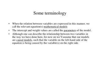
Some terminology. When the relation between variables are expressed in this manner, we call the relevant equation(s) mathematical models The intercept and weight values are called the parameters of the model.

Some terminology
E N D
Presentation Transcript
Some terminology • When the relation between variables are expressed in this manner, we call the relevant equation(s) mathematical models • The intercept and weight values are called the parameters of the model. • Although one can describe the relationship between two variables in the way we have done here, for now on we’ll assume that our models are causal models, such that the variable on the left-hand side of the equation is being caused by the variable(s) on the right side.
Terminology • The values of Y in these models are often called predicted values, sometimes abbreviated as Y-hat or . Why? They are the values of Y that are implied or predicted by the specific parameters of the model.
Parameter Estimation • Up to this point, we have assumed that our basic models are correct. • There are two important issues we need to deal with, however: • Is the basic model correct (regardless of the value of the parameters)? That is, is a linear, as opposed to a quadratic, model the appropriate model for characterizing the relationship between variables? • If the model is correct, what are the most right parameter values for the model?
Parameter Estimation • For now, we will continue to assume that the basic model is correct. In the third part of the course, we will deal with methods for comparing alternative models. • The process of obtaining the correct parameter values (assuming we are working with the right model) is called parameter estimation.
Parameter Estimation • Often, theories specify the form of the relationship rather than the specific values of the parameters • The parameters themselves, assuming the basic model is correct, are typically estimated from data. We refer to the estimation processes as “calibrating the model.” • We need a method for choosing parameter values that will give us the best representation of the data possible.
Parameter Estimation example • Let’s assume that we believe there is a linear relationship between X and Y. • Assume we have collected the following data • Which set of parameter values will bring us closest to representing the data accurately?
Estimation example • We begin by picking some values, plugging them into the equation, and seeing how well the implied values correspond to the observed values • We can quantify what we mean by “how well” by examining the difference between the model-implied Y and the actual Y value • this difference, , is often called error in prediction
Estimation example • Let’s try a different value of b and see what happens • Now the implied values of Y are getting closer to the actual values of Y, but we’re still off by quite a bit
Estimation example • Things are getting better, but certainly things could improve
Estimation example • Ah, much better
Estimation example • Now that’s very nice • There is a perfect correspondence between the implied values of Y and the actual values of Y
Estimation example • Whoa. That’s a little worse. • Simply increasing b doesn’t seem to make things increasingly better
Estimation example • Ugg. Things are getting worse again.
Parameter Estimation example • Here is one way to think about what we’re doing: • We are trying to find a set of parameter values that will give us a small—the smallest—discrepancy between the predicted Y values and the actual values of Y. • How can we quantify this?
Parameter Estimation example • One way to do so is to find the difference between each value of Y and the corresponding predicted value (we called these differences “errors” before), square these differences, and average them together
Parameter Estimation example • The form of this equation should be familiar. Notice that it represents some kind of average of squared deviations • This average is often called error variance. • Sometimes people simply sum the squared errors. When expressed this way, the sum is often called the sum of squared errors or SSE.
Parameter Estimation example • In estimating the parameters of our model, we are trying to find a set of parameters that minimizes the error variance. In other words, we want to be as small as it possibly can be. • The process of finding this minimum value is called least-squares estimation.
Parameter Estimation example • In this graph I have plotted the error variance as a function of the different parameter values we chose for b. Notice that our error was large at first, but got smaller as we made X larger. Eventually, the error reached a minimum and, then, began to increase again as we made X larger.
Parameter Estimation example • The minimum in this example occurred when b = 2. This is the “best” value of b, when we define “best” as the value that minimizes the error variance. • There is no other value of b that will make the error smaller. (0 is as low as you can go.)
Ways to estimate parameters • The method we just used is sometimes called the brute force or gradient descent method to estimating parameters. • More formally, gradient decent involves starting with viable parameter value, calculating the error using slightly different value, moving the best guess parameter value in the direction of the smallest error, then repeating this process until the error is as small as it can be. • Analytic methods • With simple linear models, the equation is so simple that brute force methods are unnecessary.
Analytic least-squares estimation • Specifically, one can use calculus to find the values of a and b that will minimize the error function
Analytic least-squares estimation • When this is done (we won’t actually do the calculus here ), the obtain the following equations:
Analytic least-squares estimation • Thus, we can easily find the least-squares estimates of a and b from simple knowledge of (1) the correlation between X and Y, (2) the SD’s of X and Y, and (3) the means of X and Y:
A neat fact • Notice what happens when X and Y are in standard score form • Thus,
In this past example, we have dealt with a situation in which a linear model of the form Y = 2 + 2X perfectly accounts for the data. (That is, there is no discrepancy between the values implied by the model and the actual data.) • When this is not true, we can still find least squares estimates of the parameters.