Download
1 / 40
400 likes | 547 Views
Some Introductory Statistics Terminology. Descriptive Statistics. Procedures used to summarize, organize, and simplify data (data being a collection of measurements or observations) taken from a sample Examples: Expressed on a 1 to 5 scale, the average satisfaction score was 3.7

E N D
Descriptive Statistics • Procedures used to summarize, organize, and simplify data (data being a collection of measurements or observations) taken from a sample • Examples: • Expressed on a 1 to 5 scale, the average satisfaction score was 3.7 • 43% of students in an online course cited that family obligations were the main motivation behind choosing distance education
Inferential Statistics • Techniques that allow us to make inferences about a population based on data that we gather from a sample • Study results will vary from sample to sample strictly due to random chance (i.e., sampling error) • Inferential statistics allow us to determine how likely it is to obtain a set of results from a single sample • This is also known as testing for “statistical significance”
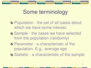
Population • A population is the entire set of individuals that we are interested in studying • This is the group that we want to generalize, or apply, our results to • Although populations can vary in size, they are usually quite large • Thus, it is usually not feasible to collect data from the entire population
Sample • A sample is simply a subset of individuals selected from the population • In the best case, the sample will be representative of the population • That is, the characteristics of the individuals in the sample will mirror those in the population
Variables • A characteristic that takes on different values for different individuals in a sample • Examples: • Gender • Age • Course satisfaction • The amount of instructor contact during the semester
Independent Variables (IV) • The “explanatory” variable • The variable that attempts to explain or is purported to cause differences in a second variable • Example: • Does the use of a computer-delivered curriculum enhance student achievement? • Whether or not (yes or no) students received the computer instruction is the IV
Dependent Variables (DV) • The “outcome” variable • The variable that is thought to be influenced by the independent variable • Example: • Does the use of a computer-delivered curriculum enhance student achievement? • Student achievement is the DV
Confounding Variables • Researchers are usually only interested in the relationship between the IV and DV • Confounding variables represent unwanted sources of influence on the DV, and are sometimes referred to as “nuisance” variables • Example: • Does the use of a computer-delivered curriculum enhance student achievement? • One’s previous experience with computers, age, gender, SES, etc. may all be confounding variables
Controlling Confounding Variables • Typically, researchers are interested in excluding, or controlling for, the effects of confounding variables • This is not a statistical issue, but is accomplished by the research design • Certain types of designs (e.g., true experiments) better control the effects of confounding variables
Measures of Central Tendency • Three measures of central tendency are available • The Mean • The Median • The Mode • Unfortunately, no single measure of central tendency works best in all circumstances • Nor will they necessarily give you the same answer
Example • SAT scores from a sample of 10 college applicants yielded the following: • Mode: 480 • Median: 505 • Mean: 526 • Which measure of central tendency is most appropriate?
The Mean • The mean is simply the arithmetic average • The mean would be the amount that each individual would get if we took the total and divided it up equally among everyone in the sample • Alternatively, the mean can be viewed as the balancing point in the distribution of scores (i.e., the distances for the scores above and below the mean cancel out)
The Median • The median is the score that splits the distribution exactly in half • 50% of the scores fall above the median and 50% fall below • The median is also known as the 50th percentile, because it is the score at which 50% of the people fall below
Special Notes • A desirable characteristic of the median is that it is not affected by extreme scores • Example: • Sample 1: 18, 19, 20, 22, 24 • Sample 2: 18, 19, 20, 22, 47 • The median is 20 in both samples • Thus, the median is not distorted by skewed distributions
The Mode • The mode is simply the most common score • There is no formula for the mode • When using a frequency distribution, the mode is simply the score (or interval) that has the highest frequency value • When using a histogram, the mode is the score (or interval) that corresponds to the tallest bar
Choosing the Proper Statistic • Continuous data • Always report the mean • If data are substantially skewed, it is appropriate to use the median as well • Categorical data • For nominal data you can only use the mode • For ordinal data the median is appropriate (although people often use the mean)
Distribution Shape and Central Tendency • In a normal distribution, the mean, median, and mode will be approximately equal
Distribution Shape (2) • In a skewed distribution, the mode will be the peak, the mean will be pulled toward the tail, and the median will fall in the middle
Overview • After collecting data, researchers are faced with pages of unorganized numbers, stacks of survey responses, etc. • The goal of descriptive statistics is to aggregate the individual scores (datum) in a way that can be readily summarized • A frequency distribution table can be used to get “picture” of how scores were distributed
Frequency Distributions • A frequency distribution displays the number (or percent) of individuals that obtained a particular score or fell in a particular category • As such, these tables provide a picture of where people respond across the range of the measurement scale • One goal is to determine where the majority of respondents were located
When To Use Frequency Tables • Frequency distributions and tables can be used to answer all descriptive research questions • It is important to always examine frequency distributions on the IV and DV when answering comparative and relationship questions
Three Components of a Frequency Distribution Table • Frequency • the number of individuals that obtained a particular score (or response) • Percent • The corresponding percentage of individuals that obtained a particular score • Cumulative Percent • The percentage of individuals that fell at or below a particular score (not relevant for nominal variables)
Example (1) • Frequency distribution showing the ages of students who took the online course
Example (2) • Student responses when asked whether or not they would recommend the online course to others • Most would recommend the course
Independent t-Test • The independent samples t-test is used to test comparative research questions • That is, it tests for differences in two group means • Two groups are compared on a continuous DV
Scenario • Suppose we wish to compare how males and females differed with respect to their satisfaction with an online course • The null hypothesis states that men and women have identical levels of satisfaction
Research Question • If we were conducting this study, the research question could be written as follows: • Are there differences between males and females with respect to satisfaction? • The word “differences” was used to denote a comparative question
The Data (1) • Satisfaction is measured on a 25-point scale that ranges between 5 (low) and 30 (high) • The descriptive statistics were as follows:
The Data (2) • On a 25-point satisfaction scale, men and women differed by about 5 points (means were 18.75 and 23.5, respectively) • They were not identical, but how likely is a 5 point difference to occur from the hypothetical population where men and women are identical?
Conceptual Formula • The conceptual formula for the t statistic is • The formula tells how big the 5 point difference we observed is relative to the difference expected simply due to sampling error
Results • The t-statistic value was 1.695, suggesting that the 5-point difference is not quite twice as large as the difference we would expect due to chance (which is quantified by the standard error statistic) • The p-value for the analysis was .116 (almost .12, or 12%)
Interpreting the Probability • Thus, there was about a 12% chance that this sample (the 5 point difference) originated from the hypothetical null hypothesis population • The p-value is greater than .05, so we would retain the null (results are not significant) • Thus, there is no evidence that males and females differ in their satisfaction
Cohen’s d Effect Size • Recall that p-values don’t tell how important the results are • A measure of effect size can be computed that helps us quantify the magnitude of the results we obtained • The mean difference (5 points) is expressed in standard deviation units
Example • Using the statistics from the SPSS printout, the d effect size can be computed as
Interpreting Cohen’s d • Cohen (1988) suggested the following guidelines for interpreting the d effect size • d > .20 is a small effect size (1/5 of a standard deviation difference) • d > .50 is a medium effect size (1/2 of a standard deviation difference) • d > .80 is a large effect size (4/5 of a standard deviation difference)
Writing Up the Results • If you were writing the results for publication, it could go something like this: • “As seen in Table 1, satisfaction scores for female students were approximately five points higher, on average, than those of males. Using an independent t test, no statistically significant differences were observed between the group means, (t (12) = 1.70, p = .12). However, despite no statistical significance, Cohen’s d effect size indicated a large difference between the groups (d = .92)”