Download
1 / 68
720 likes | 1.4k Views
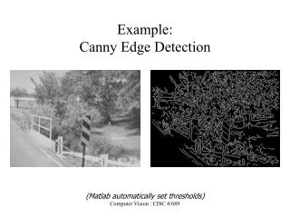
Example: Canny Edge Detection. (Matlab automatically set thresholds). More: facts and figures. The convolution of two Gaussians with variances { 1 } 2 and { 2 } 2 is { 1 } 2 +{ 2 } 2 . This is same as consecutive smoothing with the two corresponding SD’s.

E N D
Example: Canny Edge Detection (Matlab automatically set thresholds) Computer Vision : CISC 4/689
More: facts and figures • The convolution of two Gaussians with variances {1}2 and {2}2 is {1}2+{2}2. This is same as consecutive smoothing with the two corresponding SD’s. • Thus, generic formula is: i{i}2 • Problem: A discrete appx. to a 1D Gaussian can be obtained by sampling g(x). In practice, samples are taken uniformly until the truncated values at the tails of the distribution are less than 1/1000 of the peak value. a) For =1, show that the filter is 7 pixels wide. Computer Vision : CISC 4/689
Answer.. • Lets pick (n+1) pixels from the center of kernel(including center). This way, total kernel size is 2n+1, n pixels on either side of origin. Exp(-{(n+1)2}/{22}) < 1/1000 So, n > 3.7 -1 n must be the nearest integer to 3.7 -0.5 For =1, n=3, 2n+1=7. Filter coefficients can be obtained as {-3,-2,-1,0,1,2,3} Computer Vision : CISC 4/689
Choice of • The choice of depends on the scale at which the image is to be displayed. • Small values bring out edges at a fine scale, vice-versa. • Noise is another factor to look into the selection, along with computational cost Computer Vision : CISC 4/689
Some comparisons Zero-crossings easy to find than threshold Computer Vision : CISC 4/689
Canny • Many implementations of the Canny edge detector approximate this process by first convolving the image with a Gaussian to smooth the signal, and then looking for maxima in the first partial derivatives of the resulting signal (using masks similar to the Sobel masks). • Thus we can convolve the image with 4 masks, looking for horizontal, vertical and diagonal edges. The direction producing the largest result at each pixel point is marked. • Record the convolution result and the direction of the edge at each pixel. Computer Vision : CISC 4/689
Marr-Hildreth vs. Canny • Laplacian is isotropic, computationally efficient: single convolution, look for zero-crossing. (one way to explain zero-crossing is, if first derivative can be looked at as a function, its maximum will be its derivative=0). • Canny being a directional operator (derivative in 4 or 3 directions), more costly, esp. due to hysterisis. • Two derivatives -> more sensitive to noise Computer Vision : CISC 4/689
Image Pyramids • Observation: Fine-grained template matching expensive over a full image • Idea: Represent image at smaller scales, allowing efficient coarse- to-fine search • Downsampling: Cut width, height in half at each iteration: from Forsyth & Ponce Computer Vision : CISC 4/689
Gaussian Pyramid • Let the base (the finest resolution) of an n-level Gaussian pyramid be defined as P0=I. Then the ith level is reduced from the level below it by: • Upsampling S"(I): Double size of image, interpolate missing pixels courtesy of Wolfram Computer Vision : CISC 4/689 Gaussian pyramid
Laplacian Pyramids • The tip (the coarsest resolution) of an n-level Laplacian pyramid is the same as the Gaussian pyramid at that level: Ln(I) =Pn(I) • The ith level is expanded from the level above according to Li(I) =Pi(I) ¡S"(Pi+1(I)) • Synthesizing the original image: Get I back by summing upsampled Laplacian pyramid levels Computer Vision : CISC 4/689
Laplacian Pyramid • The differences of images at successive levels of the Gaussian pyramid define the Laplacian pyramid. To calculate a difference, the image at a higher level in the pyramid must be increased in size by a factor of four prior to subtraction. This computes the pyramid. • The original image may be reconstructed from the Laplacian pyramid by reversing the previous steps. This interpolates and adds the images at successive levels of the pyramid beginning with the lowest level. • Laplacian is largely uncorrelated, and so may be represented pixel by pixel with many fewer bits than Gaussian. courtesy of Wolfram Computer Vision : CISC 4/689
Reconstruction Computer Vision : CISC 4/689
Splining • Build Laplacian pyramids LA and LB for A & B images • Build a Gaussian pyramid GR from selected region R • Form a combined pyramid LS from LA and LB using nodes of GR as weights: LS(I,j) = GR(I,j)*LA(I,j)+(1-GR(I,j))*LB(I,j) Collapse the LS pyramid to get the final blended image Computer Vision : CISC 4/689
Splining (Blending) • Splining two images simply requires: 1) generating a Laplacian pyramid for each image, 2) generating a Gaussian pyramid for the bitmask indicating how the two images should be merged, 3) merging each Laplacian level of the two images using the bitmask from the corresponding Gaussian level, and 4) collapsing the resulting Laplacian pyramid. • i.e. GS = Gaussian pyramid of bitmask LA = Laplacian pyramid of image "A" LB = Laplacian pyramid of image "B" therefore, "Lout = (GS)LA + (1-GS)LB" Computer Vision : CISC 4/689
Example images from GTech Image-1 bit-mask image-2 Direct addition splining bad bit-mask choice Computer Vision : CISC 4/689
Outline • Corner detection • RANSAC Computer Vision : CISC 4/689
Matching with Invariant Features Darya Frolova, Denis Simakov The Weizmann Institute of Science March 2004 Computer Vision : CISC 4/689
Example: Build a Panorama Computer Vision : CISC 4/689 M. Brown and D. G. Lowe. Recognising Panoramas. ICCV 2003
How do we build panorama? • We need to match (align) images Computer Vision : CISC 4/689
Matching with Features • Detect feature points in both images Computer Vision : CISC 4/689
Matching with Features • Detect feature points in both images • Find corresponding pairs Computer Vision : CISC 4/689
Matching with Features • Detect feature points in both images • Find corresponding pairs • Use these pairs to align images Computer Vision : CISC 4/689
Matching with Features • Problem 1: • Detect the same point independently in both images no chance to match! We need a repeatable detector Computer Vision : CISC 4/689
Matching with Features • Problem 2: • For each point correctly recognize the corresponding one ? We need a reliable and distinctive descriptor Computer Vision : CISC 4/689
More motivation… • Feature points are used also for: • Image alignment (homography, fundamental matrix) • 3D reconstruction • Motion tracking • Object recognition • Indexing and database retrieval • Robot navigation • … other Computer Vision : CISC 4/689
Corner Detection • Basic idea: Find points where two edges meet—i.e., high gradient in two directions • “Cornerness” is undefined at a single pixel, because there’s only one gradient per point • Look at the gradient behavior over a small window • Categories image windows based on gradient statistics • Constant: Little or no brightness change • Edge: Strong brightness change in single direction • Flow: Parallel stripes • Corner/spot: Strong brightness changes in orthogonal directions Computer Vision : CISC 4/689
Corner Detection: Analyzing Gradient Covariance • Intuitively, in corner windows both Ix and Iy should be high • Can’t just set a threshold on them directly, because we want rotational invariance • Analyze distribution of gradient components over a window to differentiate between types from previous slide: • The two eigenvectors and eigenvalues ¸1,¸2 of C (Matlab: eig(C)) encode the predominant directions and magnitudes of the gradient, respectively, within the window • Corners are thus where min(¸1, ¸2) is over a threshold courtesy of Wolfram Computer Vision : CISC 4/689
Contents • Harris Corner Detector • Description • Analysis • Detectors • Rotation invariant • Scale invariant • Affine invariant • Descriptors • Rotation invariant • Scale invariant • Affine invariant Computer Vision : CISC 4/689
Window function Shifted intensity Intensity Window function w(x,y) = or 1 in window, 0 outside Gaussian Harris Detector: Mathematics Taylor series: F(x+dx,y+dy) = f(x,y) +fx(x,y)dx+fy(x,y)dy+… http://mathworld.wolfram.com.TaylorSeries.html Change of intensity for the shift [u,v]: Computer Vision : CISC 4/689
Harris Detector: Mathematics For small shifts [u,v] we have a bilinear approximation: where M is a 22 matrix computed from image derivatives: Computer Vision : CISC 4/689
Harris Detector: Mathematics Intensity change in shifting window: eigenvalue analysis 1, 2 – eigenvalues of M If we try every possible orientation n, the max. change in intensity is 2 Ellipse E(u,v) = const 1 2 Computer Vision : CISC 4/689
Harris Detector: Mathematics 2 Classification of image points using eigenvalues of M: “Edge” 2 >> 1 “Corner”1 and 2 are large,1 ~ 2;E increases in all directions 1 and 2 are small;E is almost constant in all directions “Edge” 1 >> 2 “Flat” region 1 Computer Vision : CISC 4/689
Harris Detector: Mathematics Measure of corner response: (k – empirical constant, k = 0.04-0.06) Computer Vision : CISC 4/689
Harris Detector: Mathematics 2 “Edge” “Corner” • R depends only on eigenvalues of M • R is large for a corner • R is negative with large magnitude for an edge • |R| is small for a flat region R < 0 R > 0 “Flat” “Edge” |R| small R < 0 1 Computer Vision : CISC 4/689
Harris Detector • The Algorithm: • Find points with large corner response function R (R > threshold) • Take the points of local maxima of R Computer Vision : CISC 4/689
Harris Detector: Workflow Computer Vision : CISC 4/689
Harris Detector: Workflow Compute corner response R Computer Vision : CISC 4/689
Harris Detector: Workflow Find points with large corner response: R>threshold Computer Vision : CISC 4/689
Harris Detector: Workflow Take only the points of local maxima of R Computer Vision : CISC 4/689
Harris Detector: Workflow Computer Vision : CISC 4/689
Example: Gradient Covariances Corners are whereboth eigenvalues are big from Forsyth & Ponce Detail of image with gradient covar- iance ellipses for 3 x 3 windows Full image Computer Vision : CISC 4/689
Example: Corner Detection (for camera calibration) Computer Vision : CISC 4/689 courtesy of B. Wilburn
Example: Corner Detection courtesy of S. Smith SUSAN corners Computer Vision : CISC 4/689
Harris Detector: Summary • Average intensity change in direction [u,v] can be expressed as a bilinear form: • Describe a point in terms of eigenvalues of M:measure of corner response • A good (corner) point should have a large intensity change in all directions, i.e. R should be large positive Computer Vision : CISC 4/689
Contents • Harris Corner Detector • Description • Analysis • Detectors • Rotation invariant • Scale invariant • Affine invariant • Descriptors • Rotation invariant • Scale invariant • Affine invariant Computer Vision : CISC 4/689
Tracking: compression of video information • Harris response (uses criss-cross gradients) • Dinosaur tracking (using features) • Dinosaur Motion tracking (using correlation) • Final Tracking (superimposed) Courtesy: (http://www.toulouse.ca/index.php4?/CamTracker/index.php4?/CamTracker/FeatureTracking.html) This figure displays results of feature detection over the dinosaur test sequence with the algorithm set to extract the 6 most "interesting" features at every image frame. It is interesting to note that although no attempt to extract frame-to-frame feature correspondences was made, the algorithm still extracts the same set of features at every frame. This will be useful very much in feature tracking. Computer Vision : CISC 4/689
One More.. • Office sequence • Office Tracking Computer Vision : CISC 4/689
Harris Detector: Some Properties • Rotation invariance Ellipse rotates but its shape (i.e. eigenvalues) remains the same Corner response R is invariant to image rotation Computer Vision : CISC 4/689
Intensity scale: I aI R R threshold x(image coordinate) x(image coordinate) Harris Detector: Some Properties • Partial invariance to affine intensity change • Only derivatives are used => invariance to intensity shift I I+b Computer Vision : CISC 4/689
Harris Detector: Some Properties • But: non-invariant to image scale! All points will be classified as edges Corner ! Computer Vision : CISC 4/689