Canny Edge Detection
Canny Edge Detection. CSE 6367 – Computer Vision Vassilis Athitsos University of Texas at Arlington. What Is an Edge?. An edge pixel is a pixel at a “boundary”. There is no single definition for what is a “boundary”. output1. output2. input. Image Derivatives.

Canny Edge Detection
E N D
Presentation Transcript
Canny Edge Detection CSE 6367 – Computer Vision Vassilis Athitsos University of Texas at Arlington
What Is an Edge? • An edge pixel is a pixel at a “boundary”. • There is no single definition for what is a “boundary”. output1 output2 input
Image Derivatives • We have all learned how to calculate derivatives of functions from the real line to the real line. • Input: a real number • Output: a real number • In taking image derivatives, we must have in mind two important differences from the “typical” derivative scenario: • Input: two numbers (x, y), not one number. • Input: discrete (integer pixel coordinates). • Output: Integer between 0 and 255.
Directional Derivative • Let f(x, y) be a function mapping two real numbers to a real number. • Let theta be a direction (specified as an angle from the x axis). • Let (x1, y1) be a specific point on the plane. • Define g(x) = f(x1 + x cos(theta), y1 + x sin(theta)). • Then, g(x) is a function from the real line to the real line. • The directional derivative of f at x1, y1 is defined to be g’(0).
dx, dy Directional Derivatives • For the directional derivative of f along the x axis, we use notation df/dx. • For the directional derivative of f along the y axis, we use notation df/dy.
Vertical and Horizontal Edges • Consider the image as a function f(i,j) mapping pixels to intensity values. • Function f(i,j) can be seen as a discretized version of a more general function g(y,x), mapping pairs of real numbers to intensity values. • Vertical edges correspond to points in g with high dg/dx. • Horizontal edges correspond to points in g with high dg/dy.
Approximating dg/dx via Filtering • In the discrete domain of f(i,j), dg/dx is approximated by filtering with the right kernel: • Interpreting imfilter(gray, dx): • Results far from zero (positive and negative) correspond to strong vertical edges. • These are mapped to high positive values by abs. • Results close to zero correspond to weak vertical edges, or no edges whatsoever. dx = [-1 0 1; -2 0 2; -1 0 1]; dx = dx / (sum(abs(dx(:)))); dxgray = abs(imfilter2(gray, dx));
Result: Vertical/Horizontal Edges gray = read_gray('data/hand20.bmp'); dx = [-1 0 1; -2 0 2; -1 0 1]; dx = dx / (sum(abs(dx(:)))); dy = dx’; % dy is the transpose of dx dxgray = abs(imfilter(gray, dx, 'symmetric', 'same')); dygray = abs(imfilter(gray, dy, 'symmetric', 'same')); gray dxgray (vertical edges) dygray (horizontal edges)
Blurring and Filtering • To suppress edges corresponding to small-scale objects/textures, we should first blur. % generate two blurred versions of the image, see how it % looks when we apply dx to those blurred versions. filename = 'data/hand20.bmp'; gray = read_gray(filename); dx = [-1 0 1; -2 0 2; -1 0 1] / 8; dy = dx'; blur_window1 = fspecial('gaussian', 19, 3.0); % std = 3 blur_window2 = fspecial('gaussian', 37, 6.0); % std = 6 blurred_gray1 = imfilter(gray, blur_window1, 'symmetric'); blurred_gray2 = imfilter(gray, blur_window2 , 'symmetric'); dxgray = abs(imfilter(gray, dx, 'symmetric')); dxb1gray = abs(imfilter(blurred_gray1, dx , 'symmetric')); dxb2gray = abs(imfilter(blurred_gray2, dx , 'symmetric'));
Blurring and Filtering: Results • Smaller details are suppressed, but the edges are too thick. • Will be remedied in a few slides, with non-maxima suppression. gray dxgray No blurring dxb1gray Blurring, std = 3 dxb1gray Blurring, std = 6
Finding Edges at Other Angles • Extracting edges at angle theta: • Rotate dx by theta, or • Rotate image by –theta. • Rotating filter is typically more efficient. % detecting edges with orientation 45 or 135 degrees: fcircle = read_gray('data/blurred_fcircle.bmp'); dx = [-1 0 1; -2 0 2; -1 0 1] / 8; rot45 = imrotate(dx, 45, 'bilinear', 'loose'); rot135 = imrotate(dx, 135, 'bilinear', 'loose'); edges45 = abs(imfilter(fcircle, rot45, 'symmetric')); edges135 = abs(imfilter(fcircle, rot135, 'symmetric'));
Results: Edges at Degrees 45/135 fcircle edges135 edges45
More Edges at 45/135 Degrees original image edges at 45 degrees edges at 135 degrees
Computing Gradient Norms • Let: • dxA = imfilter(A, dx); • dyA = imfilter(A, dy); • Gradient norm at pixel (i,j): • The norm of vector (dxA(i,j), dyA(i,j)). • sqrt(dxA(i,j)^2 + dyA(i,j)^2). • The gradient norm operation identifies pixels at all orientations. • Also useful for identifying smooth/rough textures.
Computing Gradient Norms: Code • See following functions online: • gradient_norms • blur_image gray = read_gray('data/hand20.bmp'); dx = [-1 0 1; -2 0 2; -1 0 1] / 8; dy = dx'; blurred_gray = blur_image(gray, 1.4 1.4); dxgray = imfilter(blurred_gray, dx, 'symmetric'); dygray = imfilter(blurred_gray, dy, 'symmetric'); % computing gradient norms grad_norms = (dxb1gray.^2 + dyb1gray.^2).^0.5;
Gradient Norms: Results gray grad_norms dxgray dygray
Notes on Gradient Norms • Gradient norms detect edges at all orientations. • However, gradient norms in themselves are not a good output for an edge detector: • We need thinner edges. • We need to decide which pixels are edge pixels.
Non-Maxima Suppression • Goal: produce thinner edges. • Idea: for every pixel, decide if it is maximum along the direction of fastest change. • Preview of results: gradient norms result of nonmaxima suppression
Nonmaxima Suppression Example • Example: img = [112 118 111 115 112 115 112 120 124 128 128 126 128 126 132 134 132 130 130 130 130 167 165 163 162 161 162 161 190 192 199 196 198 196 198 203 205 203 205 207 205 207 212 214 216 219 216 213 217]; grad_norms = round(gradient_norms(img)); grad_norms = [ 5 5 7 7 7 7 7 10 9 9 9 8 8 9 23 21 18 17 17 17 17 29 30 32 33 34 34 34 19 20 20 22 22 22 23 11 11 10 10 10 9 9 5 5 6 6 5 4 5]; img grad_norms
Nonmaxima Suppression Example • Should we keep pixel (3,3)? • result of dx filter [-0.5 0 0.5] • (img(3,4) – img(3, 2)) / 2 = -2. • result of dy filter [-0.5; 0; 0.5] • (img(4,3) – img(2, 3)) / 2 = 17.5. • Gradient = (-2, 17.5). • Gradient direction: • atan2(17.5, -2) = 1.68 rad = 96.5 deg. • Unit vector at gradient direction: • [0.9935, -0.1135] (y direction, x direction) img grad_norms
Nonmaxima Suppression Example • Should we keep pixel (3,3)? • Gradient direction: 96.5 degrees • Unit vector: disp = [0.9935, -0.1135]. • disp defines the direction along which pixel(3,3) must be a local maximum. • Positions of interest: • [3,3] + disp, [3,3] – disp. • We compare grad_norms(3,3) with: • grad_norms(3.9935, 2.8865), and • grad_norms(2.0065, 3.1135) img grad_norms
Nonmaxima Suppression Example • We compare grad_norms(3,3) with: • grad_norms(3.9935, 2.8865), and • grad_norms(2.0065, 3.1135) • grad_norms(3.9935, 2.8865) = ? • Use bilinear interpolation. • (3.9935, 2.8865) is surrounded by: • (3,2) at the top and left. • (3,3) at the top and right. • (4,2) at the bottom and left. • (4,3) at the bottom and right. img grad_norms
Nonmaxima Suppression Example • grad_norms(3.9935, 2.8865) = ? • Weighted average of surrounding pixels. • See function bilinear_interpolation online. img top_left = image(top, left); top_right = image(top, right); bottom_left = image(bottom, left); bottom_right = image(bottom, right); wy = 3.9935 – 3 = 0.9935; wx = 2.8865 – 2 = 0.8865; result = (1 – wx) * (1 – wy) * top_left + wx * (1 - wy) * top_right + (1 – wx) * y * bottom_left + x * y * bottom_right; grad_norms
Nonmaxima Suppression Example • grad_norms(3.9935, 2.8865) = 33.3 • grad_norms(2.0065, 3.1135) = 10.7 • grad_norms(3,3) = 18 • Position 3,3 is not a local maximum in the direction of the gradient. • Position 3,3 is set to zero in the result of non-maxima suppression • Same test applied to all pixels. img grad_norms
Nonmaxima Suppression Result img grad_norms grad_norms = [ 5 5 7 7 7 7 7 10 9 9 9 8 8 9 23 21 18 17 17 17 17 29 30 32 33 34 34 34 19 20 20 22 22 22 23 11 11 10 10 10 9 9 5 5 6 6 5 4 5]; nonmaxima_suppression(grand_norms, thetas, 1) = [ 0 0 0 0 0 0 0 0 0 0 0 0 0 0 0 0 0 0 0 0 0 0 29 34 33 34 33 0 0 0 0 0 0 0 0 0 0 0 0 0 0 0 0 0 0 0 0 0 0 result of non-maxima suppression
Nonmaxima Suppression Result gradient norms result of nonmaxima suppression
Side Note: Bilinear Interpolation • grad_norms(3.9935, 2.8865) = ? • Weighted average of surrounding pixels. • Interpolation is a very common operation. • Images are discrete, sometimes it is convenient to treat them as continuous values. top_left = image(top, left); top_right = image(top, right); bottom_left = image(bottom, left); bottom_right = image(bottom, right); wy = 3.9935 – 3 = 0.9935; wx = 2.8865 – 2 = 0.8865; result = (1 – wx) * (1 – wy) * top_left + wx * (1 - wy) * top_right + (1 – wx) * y * bottom_left + wx * wy * bottom_right;
bilinear_interpolation.m function result = bilinear_interpolation(image, row, col) % row and col are non-integer coordinates, and this function % computes the value at those coordinates using bilinear interpolation. % Get the bounding square. top = floor(row); left = floor(col); bottom = top + 1; right = left + 1; % Get values at the corners of the square top_left = image(top, left); top_right = image(top, right); bottom_left = image(bottom, left); bottom_right = image(bottom, right); x = col - left; y = row - top; result = (1 - x) * (1 - y) * top_left; result = result + x * (1 - y) * top_right; result = result + x * y * bottom_right; result = result + (1 - x) * y * bottom_left;
The Need for Thresholding • Many non-zero pixels in the result of nonmaxima suppression represent very weak edges. gray nonmaxima nonmaxima > 0
The Need for Thresholding • Decide which are the edge pixels: • Reject maxima with very small values. • Hysteresis thresholding. gray gradient norms result of nonmaxima suppression
Hysteresis Thresholding • Use two thresholds, t1 and t2. • Pixels above t2 survive. • Pixels below t1 do not survive. • Pixels >= t1 and < t2 survive if: • They are connected to a pixel >= t2 via an 8-connected path of other pixels >= t1.
Hysteresis Thresholding Example • A pixel is white in C if: • It is white in A, and • It is connected to a white pixel of B via an 8-connected path of white pixels in A. A = nonmaxima >= 4 B = nonmaxima >= 8 C = hysthresh(nonmaxima, 4, 8)
Canny Edge Detection • Blur input image. • Compute dx, dy, gradient norms. • Do non-maxima suppression on gradient norms. • Apply hysteresis thresholding to the result of non-maxima suppression. • Check out these functions online: • blur_image • gradient_norms • gradient_orientations • nonmaxsup • hysthresh • canny • canny4
Side Note: Angles/Directions/Orientations • To avoid confusion, you must specify: • Unit (degrees, or radians). • Do you use undirected or directed orientation? • Undirected: 180 degrees = 0 degrees. • Directed: 180 degres != 0 degrees. • Which axis is direction 0? Pointing which way? • Class convention: direction 0 is x axis, pointing right. • Do angles increase clockwise or counterclockwise? • Class convention: clockwise. • Does the y axis point down? (in this class: yes) • What range of values do you allow/expect? • [-180, 180]? Any real number?
Side Note: Angles/Directions/Orientations thetas = atan2(dyb1gray, dxb1gray); % atan2 convention: % values: [-pi, pi] % 0 degrees: x axis, pointing left % y axis points down % values increase clockwise Confusion and bugs stemming from different conventions are extremely common. When combining different code, make sure that you account for different conventions.
Side Note: Edge Orientation How is the orientation of an edge pixel defined?
Side Note: Edge Orientation • How is the orientation of an edge pixel defined? • It is the direction PERPENDICULAR to the gradient, i.e., the (dx, dy) vector for that pixel. • Typically (not always) 0 degrees = 180 degrees. • In other words, typically we do not care about the direction of the orientation.