Edge Detection
Edge Detection. 27 th Nov ember 2012 /. Edge Detection in Images. Goal: Automatically find the contour of objects in a scene. What For: Edges are significant descriptors, useful for classification, compression…. Edge Detection in Images. What is an object?


Edge Detection
E N D
Presentation Transcript
Edge Detection 27thNovember 2012 /
Edge Detection in Images • Goal: Automatically find the contour of objects in a scene. • What For: Edges are significant descriptors, useful for classification, compression…
Edge Detection in Images • What is an object? It is one of the goals of computer vision to identify objects in scenes.
Edges May Have Different Sources • Object Boundaries • Occlusions • Textures • Shading
What is an Edge • Lets define an edge to be a discontinuity in image intensity function. • Several Models • Step Edge • Ramp Edge • Roof Edge • Spike Edge • They can bethus detected asdiscontinuitiesof image Derivatives
Recall Now this is linear and shift invariant. Therefore, in discrete domain, it will be represented as a convolution Differentiation and convolution
Recall Now this is linear and shift invariant. Therefore, in discrete domain, it will be represented as a convolution We could approximate this as (which is obviously a convolution with Kernel ; it’s not a very good way to do things, as we shall see) Differentiation and convolution
Finite Difference in 2D Horizontal Vertical Discrete Approximation Convolution Kernels
A 1D Example • Take a line on a grayscale image
A 1D Example (II) • Filter the discrete image values, convolution against [1 -1]
Differentiating Filters 1D Discrete derivatives 2D Discrete derivatives (separable) t
Classical Operators : Prewitt Horizontal Differentiate Smooth Vertical
Classical Operators: Sobel Horizontal Differentiate Smooth Vertical
The Gradient Orientation • Like for continuous function, the gradient at each pixel points at the steepest intensity growth direction. • The gradient norm indicates the inclination of the intensity growth. • Matlab…..
Finite differences responding to noise Increasing noise -> (this is zero mean additive Gaussian noise)
Finite differences responding to noise Increasing noise -> (this is zero mean additive Gaussian noise)
Finite differences responding to noise Increasing noise -> (this is zero mean additive Gaussian noise)
Generally expect pixels to “be like” their neighbors surfaces turn slowly relatively few reflectance changes Generally expect noise processes to be independent from pixel to pixel and with zero mean Implies that smoothingsuppresses noise, (i.i.d. noise!) Gaussian Filtering the parameter in the symmetric Gaussian as this parameter goes up, more pixels are involved in the average and the image gets more blurred and noise is somehow suppressed Smoothing reduces noise
Generally expect pixels to “be like” their neighbors surfaces turn slowly relatively few reflectance changes Generally expect noise processes to be independent from pixel to pixel and with zero mean Implies that smoothingsuppresses noise, (i.i.d. noise!) Gaussian Filtering the parameter in the symmetric Gaussian as this parameter goes up, more pixels are involved in the average and the image gets more blurred and noise is somehow suppressed Smoothing reduces noise
Low - Pass The effects of smoothing Each row shows smoothing with gaussians of different width; each column shows different realisations of an image of gaussian noise.
Gradient Magnitude and edge detectors Gradient Magnitute is not a binary image -> “shows edges” but “does not allow to identify them” yet
Detecting Edges in Image • Sobel Edge Detector Threshold Discrete Derivatives Gradient Norms Edges Threshold Image I any alternative ?
Canny Edge Detector Criteria • Good Detection: The optimal detector must minimize the probability of false positives as well as false negatives. • Good Localization: The edges detected must be as close as possible to the true edges. • Single Response Constraint: The detector must return one point only for each edge point.similar to gooddetectionbutrequires an ad-hoc formulation to getrid of multiple responses to a single edge Too many responses Poor localization True Edge Poor robustness to noise
Canny Edge Detector • Basically 3 steps • Convolution with derivative of Gaussian • Non-maximum Suppression • Hysteresis Thresholding J. Canny “A Computational Approach to Edge Detection” IEEE PAMI vol 8, no. 6, Nov. 1986 http://perso.limsi.fr/Individu/vezien/PAPIERS_ACS/canny1986.pdf
Canny Edge Detector • Smooth by Gaussian • Compute x and y derivatives • Compute gradient magnitude and orientation
An Overview on Threshold • According to the way the Threshold T is used/determined they are divided into • Global Threshold • Local (or) Adaptive Threshold • According to the output they can be classified in • Binary Threshold • Hard Threshold • Soft Threshold • Matlab…
Non-Maximum Suppression: The Idea • We wish to determine the points along the curve where the gradient magnitude is largest. • Non-maximum suppression: we look for a maximum along a slice orthogonal to the curve. These points form a 1D curve. • There are two issues: • which point is the maximum, • and where is the next one? GradientMagnitude Segmentorthogonal Original Image
Non-Maximum Suppression: Quantize Gradient Directions • For each pixel compute gradientdirection and quantizeit in 4 maindirection, eachcovering 45° (orientationisnotconsidered) • For each pixel buld up a segmentfollowing the quantizeddirections 0,1,2,3 06/12/2011
Non-Maximum Suppression – Idea (II) A segmentorthogonal to the gradientdirection in a pixel The intensityprofilealong the segment
Non-Maximum Suppression - Threshold • Suppress the pixels in ‘Gradient Magnitude Image’ which are not local maximum • These have to be taken on a line along the direction orthogonal to the gradient in (x,y)
Hysteresis Thresholding • Use of two different threshold High and Low for • For new edge starting point • For continuing edges • In such a way the edges continuity is preserved
Hysteresis Thresholding • If the gradient at a pixel is above ‘High’, declare it an ‘edge pixel’. • If the gradient at a pixel is below ‘Low’, declare it a ‘non-edge-pixel’. • If the gradient at a pixel is between ‘Low’ and ‘High’ then declare it an ‘edge pixel’ if and only if it is connected to an ‘edge pixel’ directly or via pixels between ‘Low’ and ‘ High’.
Examples its detected edges an image
In matlab.. • Canny edge detector is implemented with theedge.m command
A brief overview on Morphological Operators in Image Processing GiacomoBoracchi 24/11/2010 boracchi@elet.polimi.it
An overview on morphological operations • Erosion, Dilation • Open, Closure • We assume the image being processed is binary, as these operators are typically meant for refining “mask” images.
Erosion • General definition: Nonlinear Filtering procedure that replace to each pixel valuethe minimum on a given neighbor • As a consequence on binary images E(x)=1 iff the image in the neighbor is constantly 1 • This operation reduces thus the boundaries of binary images • It can be interpreted as an AND operation of the image and the neighbor overlapped at each pixel