Download
1 / 16
160 likes | 302 Views
Canny Edge Detector. However, usually there will still be noise in the array E[ i , j], i.e., non-zero values that do not correspond to any edge in the original image. In most cases, these values will be smaller than those indicating actual edges.

E N D
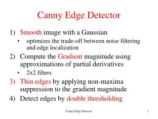
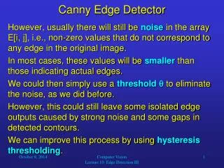
Canny Edge Detector • However, usually there will still be noise in the array E[i, j], i.e., non-zero values that do not correspond to any edge in the original image. • In most cases, these values will be smaller than those indicating actual edges. • We could then simply use a threshold to eliminate the noise, as we did before. • However, this could still leave some isolated edge outputs caused by strong noise and some gaps in detected contours. • We can improve this process by using hysteresis thresholding. Computer Vision Lecture 10: Edge Detection III
Canny Edge Detector • Hysteresis thresholding uses two thresholds - a low threshold L and a high threshold H. • Typically, His chosen so that 2L H 3L. • In the first stage, we label each pixel in E[i, j] as follows: • If E[i, j] > H then the pixel is an edge, • If E[i, j] < Lthen the pixel is no edge (deleted), • Otherwise, the pixel is an edge candidate. Computer Vision Lecture 10: Edge Detection III
Canny Edge Detector • In the second stage, we check for each edge candidate c whether it is connected to an edge via other candidates (8-neighborhood). • If so, we turn c into an edge. • Otherwise, we delete c, i.e., it is no edge. • This method fills gaps in contours and discards isolated edges that are unlikely to be part of any contour. Computer Vision Lecture 10: Edge Detection III
220 219 183 170 120 78 209 215 200 180 131 101 211 202 182 119 87 71 176 165 121 101 100 82 100 105 90 84 119 69 79 85 97 77 75 58 grayscale image intensity values of same image Canny Edge Detector - Example • Let us look at the following (already smoothed) sample image and perform Canny edge detection on it: Computer Vision Lecture 10: Edge Detection III
2 -25 -16.5 -49.5 -36 0 -7 7 13.5 10.5 17 0 -1.5 -17.5 -41.5 -40.5 -23 0 -5.5 -15.5 -39.5 -52.5 -37 0 -10 -32 -41.5 -16.5 -17 0 -36 -49 -39.5 -2.5 12 0 -3 -29.5 -13 -17 -34 0 -68 -45.5 -24 1 3 0 5.5 -1.5 -13 16.5 -33.5 0 -20.5 -6.5 0 -25.5 -27.5 0 0 0 0 0 0 0 0 0 0 0 0 0 Q[i, j] P[i, j] Canny Edge Detector - Example • Applying the vertical and horizontal gradient filters gives us the following results: Computer Vision Lecture 10: Edge Detection III
7.3 26 21.3 50.6 39.8 0 164 286 309 282 295 0 5.7 23.4 57.3 66.3 43.6 0 195 228 226 218 212 0 37.4 58.5 57.3 16.7 20.8 0 196 213 226 261 305 0 68.1 54.2 27.3 17 34.1 0 183 213 208 87 275 0 21.2 6.7 13 30.4 43.3 0 165 193 270 147 231 0 0 0 0 0 0 0 0 0 0 0 0 0 m[i, j] [i, j] Canny Edge Detector - Example • Based on P[i, j] and Q[i, j], we can now compute the magnitude and orientation of the gradient: Computer Vision Lecture 10: Edge Detection III
Remember the directions: 0 2 3 2 3 0 0 1 1 1 1 0 0 1 1 2 3 0 1 0 3 0 1 1 2 2 0 2 [i,j] 2 0 0 2 3 1 0 0 0 0 0 0 0 3 0 1 [i, j] Canny Edge Detector - Example • This allows us to compute the sector [i, j] for each gradient angle [i, j]: Computer Vision Lecture 10: Edge Detection III
7.3 26 0 50.6 0 0 0 0 57.3 66.3 0 0 0 58.5 57.3 0 0 0 68.1 54.2 0 0 20.8 0 0 0 0 0 34.1 0 0 0 0 0 43.3 0 E[i, j] Canny Edge Detector - Example • Next step: nonmaxima suppression: Computer Vision Lecture 10: Edge Detection III
Canny Edge Detector - Example • Finally: hysteresis thresholding (L = 30, H= 60): 0 0 0 ? 0 0 0 0 0 1 0 0 0 0 ? 1 0 0 0 0 1 1 0 0 0 ? ? 0 0 0 0 1 1 0 0 0 1 ? 0 0 0 0 1 1 0 0 0 0 0 0 0 0 ? 0 0 0 0 0 0 0 0 0 0 0 ? 0 0 0 0 0 0 0 Hysteresis stage 1: 1 = edge; 0 = no edge; ? = edge candidate Hysteresis stage 2: 1 = edge; 0 = no edge; Computer Vision Lecture 10: Edge Detection III
edge pixels edge locations in original image Canny Edge Detector - Example • Finally we visualize the detected edge pixels (0 = black, 1 = white) and indicate the precise edge locations (the pixels’ lower right corners) in the original image: Computer Vision Lecture 10: Edge Detection III
Evaluating Edge Detector Performance • How can we decide which type of edge detector we should use in our application? • For this purpose, we need to find a method for evaluating the performance of these detectors. • First of all, we need to create one of more test images for which we know the actual locations and orientations of edges. • A straightforward idea is to just draw an image showing geometric objects. • One possible measure for edge detector performance is called the figure of merit. Computer Vision Lecture 10: Edge Detection III
Evaluating Edge Detector Performance • The figure of merit FM is computed as follows: with number of detected edges IA, number of ideal edges II, distance between the actual and ideal edges (as matched by an appropriate algorithm) d, and constant for penalizing displaced edges . Computer Vision Lecture 10: Edge Detection III
Evaluating Edge Detector Performance • The maximum value of FM is 1, which indicates perfect performance. • The closer FM is to 0, the poorer the performance. • Of course even a poor edge detector can perform very well in artificial images that show, for example, only perfect rectangles. • In order to perform a more meaningful analysis, we should add noise to our test images and see how well our edge detector can handle it. • One possibility is to simulate varying degrees of Gaussian noise in our test images. Computer Vision Lecture 10: Edge Detection III
Probability for new intensity i’ of pixel probability original intensity i of pixel intensity Simulating Gaussian Noise • In order to simulate Gaussian noise, change the intensity of each pixel according to a Gaussian random distribution: standard deviation of Gaussian determines amount of noise Computer Vision Lecture 10: Edge Detection III
probability intensity original intensity i of pixel new intensity i’ Simulating Gaussian Noise • To simulate a Gaussian random distribution, keep on choosing 2D random points in the marked rectangular area until one of them is under the Gaussian curve. • Set i’ to the horizontal coordinate of that point. Computer Vision Lecture 10: Edge Detection III
1 strong (robust) edge detector figure of merit weak edge detector 0 0 50 100 of Gaussian noise Evaluating Edge Detector Performance • We can then measure the figure of merit as a function of the Gaussian noise added to the input image: Computer Vision Lecture 10: Edge Detection III