Download
1 / 21
210 likes | 390 Views
TEMPORAL TRENDS OF MICROWAVE EMISSION FROM FOREST AREAS OBSERVED FROM SATELLITE. Simonetta Paloscia , Emanuele Santi, Simone Pettinato, Marco Brogioni CNR-IFAC, Florence Paolo Ferrazzoli, Rachid Rahmoune DISP, Tor Vergata University , Rome (Italy). Introduction.

E N D
TEMPORAL TRENDS OF MICROWAVE EMISSION FROM FOREST AREAS OBSERVED FROM SATELLITE Simonetta Paloscia, Emanuele Santi, Simone Pettinato, Marco BrogioniCNR-IFAC, Florence Paolo Ferrazzoli, Rachid RahmouneDISP, Tor Vergata University, Rome (Italy)
Introduction • Microwave satellites demonstrated to be good sensors for investigating land surface features, and in particular soil moisture and vegetation cover, at both global and regional scales. • The retrieval of information on forests is crucial for all studies concerning global changes and carbon balance. • The temporal trends microwave emission measured by AMSR-E (Advanced Microwave Scanning Radiometer onboard Aqua) and ESA/SMOS (Soil Moisture Ocean Salinity) satellites were analyzed on some forest plots in Russia, China and Italy.
AMSR-E & SMOS data • AMSR-E data (55°) at C (6.8GHz), X (10GHz), Ku (19GHz), and Ka (37GHz) bands, were collected during one year from May 2007 to April 2008 • SMOS LC1 data al L (1.4GHz) band were collected from January to December 2010 and averaged between 37.5° and 47.5°. Samples affected by RFI were removed. • Seasonal trends of brightness temperatures (Tb) at different frequencies, in both H and V polarizations, were analyzed on the 3 test areas, together with the following microwave indexes: • Polarization Index: PI=(Tbv-Tbh)/0.5*(Tbv+Tbh) at both X- and Ku-bands; • Frequency Index: FI = [(TbvKu - TbvKa)+ (TbhKu + TbhKa)]/2; • Normalized Temperature: Tn=Tbh(C)/Tbv(Ka) or Tb(L)/Ts
Global Monitoring The following 3 forest areas, have been studied by using the AMSR-E & SMOS sensors: • A Needle-leaved deciduous forest of Larix (Jiagedaqi) in China, characterized by cold winter with snowfalls (123°E/49.8°N); • A boreal Evergreen Spruce forest in Russia, with cold winters and snowfalls (60°E/50.5°N) • The ForesteCasentinesi in Italy, a mixed forest located in Central Italy and characterized by mild weather conditions (11.8°E/43.8°N) The first 2 areas have already been selected in the past for investigations carried out by using SSM/I data
1 2 3 • Russian forest (Evergreen) • Jagedaqi forest (China) • Foreste Casentinesi (Italy) EcoClimap(% forest cover)
Jagedaqui (China) FI PI • PI(X&Ku) shows a decreasing behavior in summer, due to the increase in leaf biomass, and an increasing trend in winter, due to the simultaneous decrease of biomass and presence of snow. • The trend of LAIhas an opposite trend with respect to these curves. • The FI(Ku-Ka) shows 2 peaks, one in agreement with the development of tree LAIin summer, and the second one with snowfall in winter. LAI
FI LAI Jagedaqui (China) PI(Ku) & FI(Ku-Ka) vs. LAI PI • PI(Ku)=0.01-0.0015 LAI (R2=0.59) • FI(Ku-Ka)=0.73-1.34 (R2=0.6) • Winter data (snow) were not considered Late snowfall LAI
Jagedaqui (China) Tn(TbhC/TbvKa) vs. Rainfall • Tn=0.986-0.0023 R (R2=0.79) • Monthly rainfall data were recorded at a nearby meteo station and compared to averaged Tb data • Winter data (snow) were not considered
Jagedaqui (China) SMOS Tb data (L-band, 1.4 GHz) • SMOS Tb, normalized to surface temperatures estimated by ECMWF, was transformed into surface emissivity (Tn) • In winter (until DoY 80) the soil is frozen and covered by snow, with low permittivity and then emissivity is high. • Between DoY 90 and 120 there is a clear decreasing trend, associated to snow melting. • This effect is due to the strong variation of soil properties, from frozen to wet. • After this date, Tn increases again and shows variations partially related to soil moisture effects. Tn SMC Melting
Russia PI FI • The snowfalls in winter affect both PI and FI. • FIshows a great sensitivity to snow but even to the variations of LAI in summer and spring time. • The variations of PI at X and Ku band are similar to those in Jagedaqui. LAI
Russia PI(Ku) vs. LAI (Ecoclimap) PI LAI • PI(Ku)=0.007-0.0012 LAI (R2=0.56) • Winter data (snow) were not considered
RussiaTn(TbhC/TbvKa) vs. Rainfall • Tn=0.99-0.0003 R (R2=0.57) • Monthly rainfall data were recorded at a nearby meteo station and compared to averaged Tb data • Winter data (snow) were not considered
RussiaSMOS Tb data (L-band, 1.4 GHz) • In winter (until DoY 80) SMOS surface emissivity, Tn, shows values close to 1, when the soil is frozen and covered by snow, with low permittivity. • Between DoY 80 and 120 there is a clear decreasing trend, associated to snow melting. • This effect is due to the strong variation of soil properties, from frozen to wet. • However, the emissivity remains > 0.9 and does not show further variations related to soil moisture effects, due to the high forest density. Tn SMC Melting
Casentino (Italy) • A mixed dense forest located in Tuscany, was selected as a temperate test area, where snowfalls are rather exceptional. • Due to the small dimensions and the heterogeneity of the area, a preliminary analysis was carried out by using a RGB Landsat image in order to better identify and geolocate the forest site. • The dimensions of the image are 40kmx40km. In the image, the area of about 20 km x 20km, corresponding to the AMSR-E acquisition, was indicated. RGB Landsat image in the visible bands: R= Band 3 (0.63-0.69 m) G= Band 2 (0.53-0.61 m) B= Band 1 (0.45-0.52 m)
Casentino FI, LAI PIKu • Seasonal trends of the PI(Ku),FI, andLAI from 2006 to 2008. The annual trend of FI is in phase with the forest LAI, whereas the PI(Ku) is inversely related to it. • The X-band values were not used, since they were affected by strong RFI, probably originated by the radio transmitters close to this area.
FI LAI Casentino PI(Ku) & FI(Ku-Ka) vs. LAI PI LAI • PI(Ku)=0.012-0.0009 LAI (R2=0.4) • FI(Ku-Ka)=0.98-1.44 (R2=0.65)
Sensitivity to SMCAirborne L-band sensor • Emissivity data at L band collected with an airborne sensor on some dense forests in Tuscany showed a fairly high sensitivity to SMC at both H and V pol. • These trends have been confirmed by model simulations (Della Vecchia et al. 2010)
Conclusions • Temporal trends of brightness temperature and related microwave indexes from AMSR-E & SMOS satellites were analyzed over three forest areas characterized by different climatic conditions and tree species. • At the higher frequencies, the frequency index between Ku and Ka bands is sensitive to the snow cycle, whereas the polarization index at both X and Ku bands is sensitive to the leaf cycle. Direct relationships between PI(Ku) and LAI, derived from ECOCLIMAP database, confirmed a high correlation between these two quantities. • Looking at SMOS data, the emissivity, obtained normalizing L band (1.4 GHz) emission to the surface temperature derived from ECMWF, shows a clear decrease, at both polarizations, which can be associated to the snow melting process and therefore to a soil moisture increase.
Russia SMOS Tb data (L-band, 1.4 GHz) • SMOS Tb, normalized to surface temperatures estimated by ECMWF, was transformed into surface emissivity • In winter (until DoY 80) the soil is frozen and covered by snow, with low permittivity and then emissivity is close to 1. • Between DoY 80 and 120 there is a clear decreasing trend, associated to snow melting. • This effect is due to the strong variation of soil properties, from frozen to wet. • However, the emissivity remains > 0.9 and does not show further variations related to soil moisture effects. Soil moisture