Download
1 / 13
130 likes | 304 Views
Contents of Chapter 6. Chapter 6 Basic Traversal and Search Techniques 6.1 Techniques for binary trees 6.2 Techniques for graphs 6.3 Connected components and spanning trees 6.4 Biconnected components and DFS 6.5 References and readings. Chap. 6 Basic Traversal and Search Techniques.

E N D
Contents of Chapter 6 • Chapter 6 Basic Traversal and Search Techniques • 6.1 Techniques for binary trees • 6.2 Techniques for graphs • 6.3 Connected components and spanning trees • 6.4 Biconnected components and DFS • 6.5 References and readings
Chap. 6 Basic Traversal and Search Techniques • Traversal vs. search • Traversal • It examines every node in the given data object instance. • Search • It may not examine all vertices.
struct treenode { Type data; struct treenode *lchild, *rchild; }; void InOrder(struct treenode *t) // t is a binary tree. Each node of t has // three fields lchild, data, and rchild. { if (t) { InOrder(t->lchild); Visit(t); InOrder(t->rchild); } } 6.1 Techniques for Binary Trees • Traversal • L (moving left), R (moving right), and D (printing the data) • Six possibilities: LDR, LRD, DLR, DRL, RDL, RLD • If left before right, three possibilities • LDR (inorder traversal) • LRD (postorder traversal) • DLR (preorder traversal) • Algorithms (Programs 6.1)
void PreOrder(struct treenode *t) // t is a binary tree. Each node of t has // three fields lchild, data, and rchild. { if (t) { Visit(t); PreOrder(t->lchild); PreOrder(t->rchild); } } void PostOrder(struct treenode *t) // t is a binary tree. Each node of t has // three fields lchild, data, and rchild. { if (t) { PostOrder(t->lchild); PostOrder(t->rchild); Visit(t); } } 6.1 Techniques for Binary Trees • Algorithms (Programs 6.2)
6.1 Techniques for Binary Trees • Example (Figures 6.1 and 6.2)
6.2 Techniques for Graphs • Breath first search (BFS) and traversal (BFT) • BFS Algorithm (Program 6.5) void BFS( int v ) // A breadth first search of G is carried out beginning at vertex v. // For any node i, visited[i]==1 if i has at vertex v. The graph G and // array visited[] are global; visited[] is initialized to zero. { int u = v; Queue q(SIZE); // q is a queue of unexplored vertices. visited[v] = 1; do { for all vertices w adjacent from u { if (visited[w] == 0) { q.AddQ(w); // w is unexplored. visited[w]=1; } } if (q.Qempty()) return; // No unexplored vertex q.DeleteQ(u); // Get first unexplored vertex. } while(1); }
6.2 Techniques for Graphs • Breath first search (BFS) and traversal (BFT) (Continued) • Example 6.1 (Figure 6.4) • Visiting order: 1,2,3,4,5,6,7,8
void BFT(struct treenode G[], int n) // Breadth first traversal of G { int i; boolean visited[SIZE]; for ( i = 1; i <= n; i ++ ) // Mark all vertices unvisited. visited[i] = 0; for ( i = 1; i <= n; i++ ) if ( !visited[i] ) BFS(i); } 6.2 Techniques for Graphs • Breath first search (BFS) and traversal (BFT) (Continued) • Breath first traversal (BFT) (Program 6.6)
void DFS(int v) // Given an undirected (directed) graph G=(V,E) with // n vertices and an array visited[] initially set // to zero, this algorithm visits all vertices // reachable from v. G and visited[] are global. { visited[v] = 1; for each vertex w adjacent from v { if ( !visited[w] ) DFS(w); } 6.2 Techniques for Graphs • Depth first search (DFS) and traversal (DFT) • DFS Algorithm (Program 6.7) • Example 6.2 • Visiting order: 1,2,4,8,5,6,3,7
6.3 Connected Components and Spanning Trees • Connected component • Maximal connected subgraph (p.116 in Section 2.6.2) • E.g., Figure 2.28 (p.116) • Spanning trees (Figure 6.5) • We can easily obtain spanning trees using BFS (or DFS)
6.4 Biconnected Components and DFS • Terms • A vertex v in a connected graph G is an articulation point iff the deletion of vertex v together with all edges incident to v disconnects the graph into two or more nonempty components. • Example 6.3 (Figure 6.6) • A graph G is biconnected iff it contains no articulation point. • E.g.) • The graph of Figure 6.6(a) is not biconnected. • The graph of Figure 6.7 is biconnected.
6.4 Biconnected Components and DFS • Biconnected components • Maximal biconnected subgraph • Figure 6.8
1 for each articulation point a { • let B1, B2, …., Bk be the biconnected • components containing vertex a; • let vi, vi a, be a vertex in Bi, 1 i k; • add to G the edges (vi, vi+1), 1 i k; • 6 } 6.4 Biconnected Components and DFS • Lemma 6.1 Two biconnected components can have at most one vertex in common and this vertex is an articulation point. • Transforming a graph G into a biconnected graph (Program 6.8) • Example 6.4 • For articulation point 3, add edges (4,10) and (10,9) • For articulation point 2, add edge (1,5) • For articulation point 5, add edge (6,7)