Download
1 / 57
570 likes | 726 Views
Constraining the Inflationary Gravitational Wave Background: CMB and Direct Detection. Nathan Miller Keating Cosmology Lab CASS Journal Club 3/13/07. References. Smith, Kamionkowski, Cooray “Direct Detection of the Inflationary Gravitational Wave Background” 2005

E N D
Constraining the Inflationary Gravitational Wave Background: CMB and Direct Detection Nathan Miller Keating Cosmology Lab CASS Journal Club 3/13/07
References • Smith, Kamionkowski, Cooray “Direct Detection of the Inflationary Gravitational Wave Background” 2005 • Smith, Peiris, Cooray “Deciphering Inflation with Gravitational Waves: CMB Polarization vs. Direct Detection with Laser Interferometers” 2006 • Chongchitnan and Efstathiou “Prospects for Direct Detection of Primordial Gravitational Waves” 2006 • Smith, Pierpaolo, Kamionkowski “A New Cosmic Microwave Background Constraint to Primordial Gravitational Waves” 2006 • Friedman, Cooray, Melchiorri “WMAP-normalized Inflationary Model Predictions and the Search for Primordial Gravitational Waves with Direct Detection Experiments”, 2006
Outline • Introduction • Comparison Between CMB and Direct Detection • What can be constrained by measurements • Foregrounds
380 kyr 13.7 Gyr
Inflation • Alan Guth, 1981 • Early exponential expansion of the universe • Solves many cosmological problems • Horizon, Flatness, Magnetic Monopole • Production of primordial gravitational waves • Only early universe scenario that produces these gravitational waves • Creates CMB B-modes • Predicts stochastic gravitational wave background with a nearly scale-invariant spectrum
Inflationary Dynamics • Inflation occurs when cosmological expansion accelerates • Driven by a spatially homogeneous scalar field, Φ, the “inflaton”
Slow-Roll Inflation Rewriting with Φ as “time” variable
Primordial Power Spectra • Power spectra are evaluated when the wavelength in question leaves the horizon • Can be parametrized by a power law with the spectral indices slowly changing as a function of wavenumber
Slow-Roll Hierarchy and Flow Equations Definition of Parameters Derivatives
Evaluating the Flow Equations • Randomly choose starting slow-roll parameters • Evolve forward in time (dN < 0) until end of inflation or reaches a late time fixed point • Evaluate Observables • If evolution reaches a late-time fixed point, calculate the observables at this point • If inflation end, evaluate the flow equations backward N e-folds from the end of inflation. Calculate the observables at this point • Exact value of N to use is unknown (reheating) so a range is used
Relating Slow-Roll to Observables • Observables can be written in terms of slow-roll parameters • 2nd order in slow-roll • C=4(ln2+γ)-5
Results of Slow-Roll Flow Equations Kinney 2002
Detection of Inflation • Indirectly through the B-mode of the CMB is a goal of next generation CMB experiments • Direct detection with future space based GW detectors has become a subject of serious study
CMB • Universe was much smaller, hotter • Photons in equilibrium with the proton/electron plasma • As universe expanded, wavelength expanded, eventually energy smaller than required to keep equilibrium in proton/electron plasma • Photons free-streamed to us today • Density perturbations before recombination give rise to photon anisotropies Boomerang 03 Flight
Gravitational Waves on the CMB • CMB B-mode or “Curl” Polarization • Generated by Primordial GWB at large (1o)angular scales • Density perturbations do not create B-modes • Detection is limited by • Lensing at small (5’) scales • Large Scale Structure • Neutrinos • Foregrounds
How a blackbody becomes polarized (Thomson scattering) Plane of Polarization electron unpolarized 100% polarized Polarization ~ cos2Θ – Quadrupole Scattering Courtesy of Brian Keating
How is the CMB polarized by GW? e- Gravitational Wavevector Courtesy of Brian Keating
GW + CMB Plasma This process leads to…. Courtesy of Brian Keating
Gravitational Waves + CMB Caldwell & Kamionkowski Temperature and Polarization caused by single wave in +z direction. Courtesy of Brian Keating
Polarization Patterns • Polarization Generation by Thomson Scattering E-mode • Density fluctuations give scalar perturbations => E-mode • Gravity Waves give tensor perturbation => B, E modes B-mode Wayne Hu Courtesy of Brian Keating
WMAP Limits NO Detection of the B mode
Future CMB Experiments Measurements of the B-mode power spectrum are the focus of future CMB grounds/balloon/space based experiments
Direct Detection • Directly measure the change in lengths caused by wave passing through • Frequency probed is about 0.1 – 1 Hz • ~ 1014 Mpc-1 • Ground and space based experiments • Only space based considered for detection of GWB
Inflationary Gravitational Wave Background and Direct Detection • Don’t measure r • Only measure tensors • Energy density of the gravitational wave background • Function of wavenumber Tensor Power Spectrum today
Michelson Interferometer • Split a single laser beam in two • Send beam over paths 90o to each other • Reflect beams back and produce an interference pattern
LISA, Space-Based Laser Interferometer • 3 Spacecrafts, each containing a reference mass • Laserbeams are directed at other 2 spacecraft’s reference masses • Spacecraft shine back their own lasers, matching phase with laser of main craft • Main craft compares light from other crafts to determine through interference pattern change in distance • Secondary craft also shine their lasers at each other to determine their own separation LISA
Direct Detection Sensitivities • Constraining inflation for 3 different possible detectors are discussed • BBO • BBO-grand (10 times more sensitive) • Ultimate DECIGO (40-100 times more sensitive)
10-18 10-20 10-22 10-24 Deci-hertz Interferometer Gravitational Wave Observatory LISA Terrestrial Detectors (e.g. LCGT) Strain [Hz-1/2] Gap 10-4 102 100 104 10-2 Frequency [Hz]
Current Limits and Projected Sensitivities Solid Lines are current limits Dashed Lines are projections
From CMB to Direct Detection • To make comparisons between CMB and Direct Detection, need relation between r and ΩGW • Simplest is extrapolating measured tensor power spectrum to DD scales • Can use slow roll to calculate variables at different scales
Extrapolation Numerical Extrapolation vs. Numerical Method
r vs. ωGW 7 Extrapolation From Slow roll
Amplitude as a function of Frequency 10-15 10-17
ΩGW Comparison 0.99 < ns(kCMB) < 1.01
Combining CMB + Direct Detection • Using both measurements of the CMB and BBO/DECIGO can probe inflaton potential with NO assumptions about power-law behavior or a model shape for the potential • Slow-roll inflation • Through Hubble Constant and Φ(N) • They also can be combined to help test the single-field consistency relation
GWB and Initial Conditions • GWB behaves as a free-streaming gas of massless particles • Similar to massless neutrinos • Adiabatic Initial Conditions • Indistinguishable from massless neutrinos • CMB/LSS constraint to number of massless neutrino species translates directly to a constraint on ΩGW • Non-Adiabatic • Effects may differ from those of massless neutrinos
Constraints on GWB amplitude from CMB/LSS CMB Data Sets: WMAP, ACBAR, CBI, VSA, BOOMERanG Galaxy Power Spectrum Data: 2dF, SDSS, and Lyman-α
Adiabatic vs. Homogeneous • Adding Galaxy Survey + Lyman-α increases uncertainty over using just CMB • Discrepancy between data sets • 95% Confidence Limit of ΩGWh2<6.9x10⁻⁶ for homogeneous initial conditions Dotted Line: only CMB data Solid Line: +Galaxies and Lyman-α Dash-Dot: +Marginalize over non-zero neutrino masses
Structure of the Potential • Trajectories of the Hubble constant as a function of N can be determined by measurements of CMB+DD • Different models satisfying observational constraints on ns, αs and large r can have much different ωgw at DD scales • How does this affect the history of H • H is related to V • Φ vs. N significantly different depending on rCMB (N0) N0
Hubble Constant Trajectories 0.15 ≤ r ≤ 0.25 Trajectories with sharp features in H(N) in the last 20 e-folds of inflations will be the first to be ruled out be BBO/DECIGO
Φ vs. N r>10-2 r<10-4
V(Φ) r=0.02 r=0.001 r<10-4 Planck CMBPol CMBPol Foreground Sensitivity Limit
Types of Inflation • Each type of inflation can predict observables in allowed range • Measurements of Ps and ns at CMB/LSS scales along with upper limits to r and αs constrain inflaton potential and derivatives at time CMB/LSS scales exited the horizon • Can use fact that 35 e-folds of inflation separate CMB/LSS and BBO/DECIGO to find potential when BBO/DECIGO scales exited the horizon
Parameter Space Occupied by Different Types of Inflation Solid-blue: Power Law Dotted Magenta: Chaotic Dot-dashed cyan: Symmetry Breaking Dashed Yellow: Hybrid Everything evaluated at CMB scales
ΩGW-nt parameter space Solid-blue: Power Law Dotted Magenta: Chaotic Dot-dashed cyan: Symmetry Breaking Dashed Yellow: Hybrid Everything evaluated at BBO/DECIGO Scales
Consistency Relation Consistency Relation
Determining R • Proposal to use both CMB and DD to constrain consistency relation • With 10% foreground contamination, CMBPol could measure R=1.0±80.0 • Determine r from CMB scales, nt from direct detection scales • Laser interferometer can measure nt to • Connecting ntBBOto ntCMB adds additional uncertainty
Uncertainty of R Uncertainty implied with ns=0.95±0.1