Download
1 / 27
270 likes | 390 Views
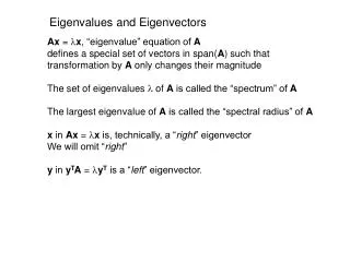
Eigenvalues and Eigenvectors. Ax = l x , “eigenvalue” equation of A defines a special set of vectors in span( A ) such that transformation by A only changes their magnitude The set of eigenvalues l of A is called the “spectrum” of A

E N D
Eigenvalues and Eigenvectors Ax = lx, “eigenvalue” equation of A defines a special set of vectors in span(A) such that transformation by A only changes their magnitude The set of eigenvalues l of A is called the “spectrum” of A The largest eigenvalue of A is called the “spectral radius” of A x in Ax = lx is, technically, a “right” eigenvector We will omit “right” y in yTA = lyT is a “left” eigenvector.
Eigenvalue equations often occur in solutions of systems of differential equations. Example: Coupled harmonic oscillators Neglecting gravity, friction, anharmonic terms, etc., the (1D) motion of a set of objects coupled by springs is determined by My + Ky = 0 where yi(t) = displacement of the ith object as a function of time. Mii = mass of ith object. Kij determines force on ith object due to displacement of object j. Look for solutions of the form yk(t) = xkeiwt Since yk(t) = -w2 xkeiwt the requirement for a solution is Ky = w2My Which has the form Ay = ly, with A = M-1K and l = w2 The solutions of Ky = w2My are called “normal modes”
Invariant subspaces: If x S implies AxS then S is called an “invariant subspace” defined by the matrix A. Sl = {x : Ax = lx} is an example of an invariant subspace, which is called the “eigenspace” of A.
Characteristic polynomial: if Ax = lx, then (A - lI)x = o (A - lI)x = o has a nonzero solution if and only if (A - lI) is singular • the eigenvalues of A are the values of l such that det(A - lI)=0 p(l) = det(A - lI) is the “characteristic polynomial” of matrix A If A is nxn then p(l) has degree n By Fundamental Theorem of Algebra, p(l) has exactly n roots (counting multiplicities) The roots of p(l) are the eigenvalues of A an nxn matrix has n eigenvalues but they may not be distinct
Example: calculate eigenvalues of det(A - lI) = det( ) = (3-l)(3-l) –1 = l2 – 6l +8 = 0 by quadratic formula l1 = 4 and l2 = 2 Even if A is a real matrix, its eigenvalues and eigenvectors may be complex Complex eigenvalues of a real matrix occur in conjugate pairs (a +i b) Eigenvalues and eigenvectors of a real symmetric matrix (most common type in models of physical systems) are real
Unless n is small, characteristic polynomial is not a useful intermediatefor eigenvalue calculation because • substantial computation required to get characteristic polynomial (2) calculation of characteristic polynomial is sensitive to round off A = has eigenvalues 1+e det(A - lI) = l2 – 2l + (1-e2) l2 – 2l + 1= (1-l)2 if e < (emach)½ (3) substantial computation required find roots of characteristic polynomial (4) No closed-form expression exist for roots of polynomial with degree > 4
Defective eigenvalues: Algebraic multiplicity of an eigenvalue is the multiplicity of its root of characteristic polynomial If p(l) has a factor (l – lk)m, then m is the algebraic multiplicity of eigenvalue lk If m = 1 then eigenvalue called “simple” Geometric multiplicity of an eigenvalue is the number of linearly independent eigenvectors associated with it Geometric multiplicity<Algebraic multiplicity Defective eigenvalues have geometric multiplicity < algebraic multiplicity Distinct eigenvalues have Geometric multiplicity = Algebraic multiplicity =1 Distinct eigenvalues of A imply “nondefective” matix A
Diagonalizable nxn matrix: If A is “nondefective” and x1, ... xn are its linearly independent eigenvectors, then matrix X formed by column vectors [x1 ... xn] has full rank and X-1 exist The collection of equations Axk = lkxk where k =1, 2,... n can be written as AX = XD where D = diag(l1,...ln) • X-1AX = D which means that A is diagonalizable Note similarity to singular-value decomposition for square matrices If A = USVT, then S = diag(s1,…sn) = UTAV = U-1AV Eigenvalues and singular values are closely related properties of A Singular values apply to non-square matrices.
Similarity Transformations: For any nonsingular matix X X-1AX is called a “similarity” transformation of A If A is nondefective, a similarity transformation exist that will determine its eigenvalues and columns of the matrix X that performs the transformation are the eigenvectors of A Eigenvalues are invariant with respect to similarity transformation Let A and B be related by a similarity transformation, then B = X-1AX det(B - lI)=det(X-1AX – l) =det(X-1AX - l X-1X) =det(X-1(A - lI)X) =det(X-1)det(A - lI)det(X) =det(A - lI) A and B have the same characteristic polynomial and same eigenvalues
If A is defective a similarity transformation that determines its eigenvalues may not exist Example: A = The solution of = (1) is x1 + x2 = x1 which implies x2 = 0 • both eigenvectors are multiples of In the absence of a 2nd linearly independent eigenvector, we cannot form a nonsingular transformation matrix X such that X-1AX is diagonal Example shows that a matrix has eigenvalues and eigenvectors even if it is not diagonalizable.
Special types of matrices: Orthogonal: ATA =AAT= I transpose is inverse Unitary: AHA =AAH= I AH means transpose and complex conjugate Symmetric: A = AT has real eigenvalues Hermitian: A = AH has real eigenvalues Normal: AHA =AAH (never defective, always has a full set of eigenvectors)
Effects of matrix modifications on its eigenvalues & eigenvectors: Shift: subtraction of constant from each diagonal element If Ax = lx then (A –sI)x = (l-s)x Eigenvalues translated by s Eigenvectors unchanged Inversion: If A is nonsingular, Ax = lx, and l 0, then A-1 x = (1/l)x. Eigenvalues of A-1 are reciprocals of eigenvalues of A Eigenvectors unchanged Powers: If Ax = lx then Ak x = lkx If p(t) = c0 + c1t + c2t2 +...+ cktk and p(A) = c0 + c1A + c2A2 +...+ ckAk then p(A)x = p(l)x. A and p(A) have the same eigenvectors
Sensitivity and Conditioning: If matrix A is subjected to a small perturbation E, how much are its eigenvalues and eigenvectors changed? Let m be the eigenvalue of A + E closest to lk • – lk is the change in eigenvalue lk due to the perturbation How is |m – lk| related to ||E|| ? |m – lk| < || X-1|| ||E||||X|| < cond(X) ||E|| eigenvalues of A are sensitive to perturbations if and only if the eigenvectors are nearly linearly dependent (i.e. if A is nearly defective) The eigenvalue problem for a normal matrix (which includes all real symmetric and complex Hermitan matrices) is always well conditioned because a normal matrix is never defective and has a full set of eigenvalues
Example of power iteration The ratio of the 2nd component on successive iterations converges (from below) to the eigenvalue of greatest magnitude Vector is converging to corresponding eigenvector
A = Normalized Power Iteration Recall that || x || = absolute value of the largest component. MatLab uses the Euclidian norm MatLab returns this eigenvector as [0.7071 0.7071]T Vectors normalized by || x || have unity for their largest component.
A = Rayleigh Quotient: Enhances convergence of power iteration If x and l are approximate eigenvectors and eigenvalues then xlAx xTxlxTAx l≈xTAx / xTx xTAx / xTx is called the Rayleigh quotient Power iteration for largest eigenvalue of
MatLab code for power iteration with accelerated convergence nxn is the dimension of A Converges to largest eigenvalue
Inverse iteration: power iteration for smallest eigenvalue Eigenvalues of A-1 are reciprocals of the eigenvalues of A • to find the smallest eigenvector of A apply power iteration to A-1 Avoid explicit inversing by solving a linear system If yk = A-1xk then Ayk = xk
A = and corresponding eigenvector
Inverse iteration with shift If Ax = lx then (A –sI)x = (l-s)x. If s is good guess for eigenvalue lk, then lk – s will be the smallest eigenvalue of A – sI • with shift, inverse iteration can be used to compute any eigenvalue and corresponding eigenvector of A using a guess obtained by some other means
MatLab code for inverse iteration with shift n = length(A(:1)); I=eye(n); sig=2; M=A-sig*I x=rand(1,n); for k=1:5 y=M\x; maxy=max(y); eigval(k)=sig+1/maxy; x=y/maxy end disp(eigval’) disp(x) x is the eigenvector normalized by absolute value of the largest component
Rayleigh Quotient Iteration Use Rayleigh quotient as approximation to an eigenvalue being refined by inverse iteration. Rapid convergence to eigenvalue with eigenvector closest x0 Note that using a new shift at each step requires LU factorization at each step • rapid convergence achieved at high cost for each step M = A – skI may become singular. Keep number of iterations small
CS 430 Spring 2014 Assignment 10, Due 4/15/14 M= • Use power iteration to find the largest eigenvalue and associated eigenvector of the matrix M. Show your Matlab code. (b) Use rayleigh quotient iteration to find the largest eigenvalue and associated eigenvector of the matrix M. Show your Matlab code (c) Use inverse iteration to find the smallest eigenvalue and associated eigenvector of M. Show your Matlab code (d) Use inverse iteration with a shift to find an eigenvalue of M with value near 2. What is the associated eigenvector? Show your Matlab code.
Chapter 8.3 pp 358,359 Computer problems 1a, 1b, 7 Computer problems 1a by characteristic polynomial Chapter 8.4 pp 368,369 Computer problems 1, 4, 6, 7