Unit 6 Analytical Vector Addition
Unit 6 Analytical Vector Addition. B. A. A. C. ½ A. Multiplying a Vector by a Scalar. A. B = 2A. C = -1/2 A. B. -B. C. A. D. Adding “-” Vectors. Add “negative” vectors by keeping the same magnitude but adding 180 degrees to the direction of the original vector. C = A + B.

Unit 6 Analytical Vector Addition
E N D
Presentation Transcript
B A A C ½ A Multiplying a Vector by a Scalar A B = 2A C = -1/2 A
B -B C A D Adding “-” Vectors • Add “negative” vectors by keeping the same magnitude but adding 180 degrees to the direction of the original vector. C = A + B D = A - B D = A + (- B)
A Ay Ax Components of Vectors A = Ax + Ay Recall: Vectors are always added “head to tail.”
Components of Vectors Finding the components when you know A. A = Ax + Ay Recall: is measured from the positive x axis.
Ax A Ay From the + x Axis If A = 3.0 m and = 45, find Ax + Ay.
Components of Vectors Finding the vector magnitude and direction when you know the components. Recall: is measured from the positive x axis. Caution: Beware of the tangent function. Always consider in which quadrant the vector lies when dealing with the tangent function.
Ax A Ay If Ax = 2.0 m and Ay. = 2.0 m, then Find A and .
Magnitude Angle Rx Ry ° ° ° Component Template Follow this type of methodology when doing these problems. 58 A=72.4m 38.37 m 61.4 m 216 B = 57.3 m -43.36 m -33.68 m 270 C = 17.8 m 0.0 m -17.80 m ii Rx = -7.99 m Ry = 9.92m R = 12.7 m Angle = 129 degrees Consider the Quadrant when using the tangent function.
1J7322 1J7322 Hand Glider Trip B = 450 m @ 135 ° C = 250 m @ 270 ° A = 300 m @ 0 °
Analytical Vector Addition – Hand Glider • Find the Final displacement of the hand glider using analytical vector addition. • This problem is similar to the following problems: WS 21, 1; WS 22, 1; and WS 23, 4. B = 450 m @ 135 ° C = 250 m @ 270 ° A = 300 m @ 0 °
Physics = Phun Analytical Vector Addition • Three Physics track robots pull on a book as shown. • They pull with the following forces: 7.0 N @ 45, 8.0 N @ 180, and 5.0 N @ 270 . • Find the net force applied to this most valuable book. • This problem is similar to WS 21, 2.
Roberts Bar & Grill Statics – Hanging Sign • Draw the Static FBD for the sign below • What do we need to do with the tension (T)? • Resolve it into its components (Tx & Ty). Ty T q T Tx Fa W
Roberts Bar & Grill Statics – Hanging Sign • Draw the Static FBD for the sign below • What do we need to do with the tension (T)? • Resolve it into its components (Tx & Ty). Ty T q T Tx Fa W Vector Addition
Inclined Plane Problems • Draw the FBD for the piano on the inclined plane. • What will we have to do with the Normal Force (N) and the force of friction (Ff)? • Resolve them into their x and y components. Ny N Ff Ffy Ffx Nx W q
Inclined Plane Problems • Would you like to do less work? • How could we do this problem by resolving only one force? • Try rotating the FBD so that the N is in the y plane and the Ff is in the x plane. N Ff Wx Wy W q Vector Addition
Analytical Vector Addition • Use the table below when performing analytical vector addition. • Do WS 23 numbers 1 & 2. Sign Problem Inclined Plane Problem
N Relative Velocity Fr Fe W N Fe W
Relative Velocity Vr Vb V Vr Vb V
Dx Vx Dy D Vy V Relative Velocity
Dx Vx Dy D Vy V Relative Velocity
H Relative Velocity
Vx Vy V Dx H Dy D Relative Velocity
Vy Dy H Dx D V Vx Relative Velocity
H Relative Velocity
Vy Dy H Dx D V Vx Relative Velocity
Relative Velocity V Vb Vb q Vr Vr
Relative Velocity V Vb Vb q Vr Vr
Vb q Vr Analytical Vector Addition • Do WS 23 number 3. • This problem is similar to WS 24, 3 and WS 22 , 2.
EIMASES This presentation was brought to you by Where we are committed to Excellence In Mathematics And Science Educational Services.
y 3-3 -x x -y Setting the Standard • When we do problems involving kinematics, it is important that we stick to a standard when imputing data into the know-want table. • This standard enables us to take into account the vector nature of acceleration, velocity, displacement, etc. • Here is a diagram we will use in order to help us correctly input data into the table. • This standard is based upon the Cartesian Coordinate system. • If a body travels West, then what sign would you give its velocity? • If a body travels at an angle of 90 degrees, then what sign would you give its velocity? 90 Degrees Up or North II I (-,+) (+,+) 180 Degrees Left or West 0 Degrees Right or East (-,-) (+,-) III IV 270 Degrees Down or South
y 3-3 -x x -y Dot Products • Write each of the three vectors given in their unit vector notation. • A = 15.0 m @ 30 • B = 22.0 m @ 225 • C = 9.0 m @ 267 • Calculate the Dot Products below. A C B
3-3 Dot Products – Finding the angle • Given the vectors below, find the angles between the following vectors. • A and C. • B and A. • C and E. • D and E.
1-17 3-D Cartisian Coordinate System +y +x +z
1-18 Unit Vectors y A = Axi + Ayj + Azk j -k -i x Note: Remember to put the “^” over the hand written vector when writing unit vectors. i k -j z
B B A A AB BA 1-19 BA = Projection of Bonto A. AB = Projection of Aonto B. Scalar or “Dot” Product The Dot product gives the projection of one vector onto another. You can also use the dot product to find the angle between the vectors.
B A 1-20 Scalar or “Dot” Product The Dot product results in a Scalar quantity.
A = Axi + Ayj B = Bxi + Byj 1-21 Scalar or “Dot” Product & Unit Vectors You “multiply” the dot product in a similar way as below. A•B = (Axi + Ayj) • (Bxi + Byj) A•B = Ax i• Bxi + Ax i•Byj+ Ayj • Bxi+ Ayj • Byj However, i • i = j • j = k • k = 1 i • j = i • k = j • k = 0 A•B = Ax Bx + AyBy
B A 1-22 Scalar or “Dot” Product One use for the dot product is to determine the angle between two vectors.
1-23 Vector or “Cross” Product The Cross product results in a VECTOR quantity. Right hand rule: Place the fingers of your right hand in the direction of the first vector in the cross product. Rotate your fingers towards the second vector. Your thumb tells you the direction of the resultant vector.
1-24 Vector or “Cross” Product The Cross product results in a VECTOR quantity. The magnitude of the vector is given by WARNING: AB sin DOES NOT EQUAL BA sin A x B DOES NOT EQUAL B x A However, A x B = - B x A
1-25 Vector or “Cross” Product AxB = (Axi + Ayj) x (Bxi + Byj) AxB = Ax ix Bxi + Ax ixByj+ Ayj x Bxi+ Ayj x Byj However, i x i = j x j = k x k = 0 i x j = -j x i = k j x k = -k x j = i K x i = -i x k = j AxB = Ax ixByj+ Ayj x Bxi AxB = (AxBy )ixj + (AyBx)j x i AxB = (AxBy )k - (AyBx)k
A = Axi + Ayj + Azk B = Bxi + Byj + Bzk 1-26 Vector or “Cross” Product Determinant method of solving for the cross product. A x B = (Axi + Ayj + Azk) x (Bxi + Byj + Bzk) A x B = AyBzi + AzBxj - AzByi + AxByk - AxBzj - AyBxk A x B = (AyBz –AzBy)i + (AzBx-AxBz)j + (AxBy-AyBx)k A x B = Rx i + Ry j + Rz k
Newton’s Laws – A Review • Newton’s First Law - An object remains at rest, or in uniform motion in a straight line, unless it is compelled to change by an externally imposed force. • Newton’s first law describes an Equilibrium Situation. • An Equilibrium Situation is one in which the acceleration of a body is equal to zero. • Newton’s Second Law – If there is a non-zero net force on a body, then it will accelerate. • Newton’s Second Law describes a Non-equilibrium Situation. • A Non-equilibrium Situation is one in which the acceleration of a body is not equal to zero. • Newton’s Third Law - for every action force there is an equal, but opposite, reaction force.