3.14 Least Squares Adaptive Filter 3.14.1 Vector Space Analysis for Least Square Filter

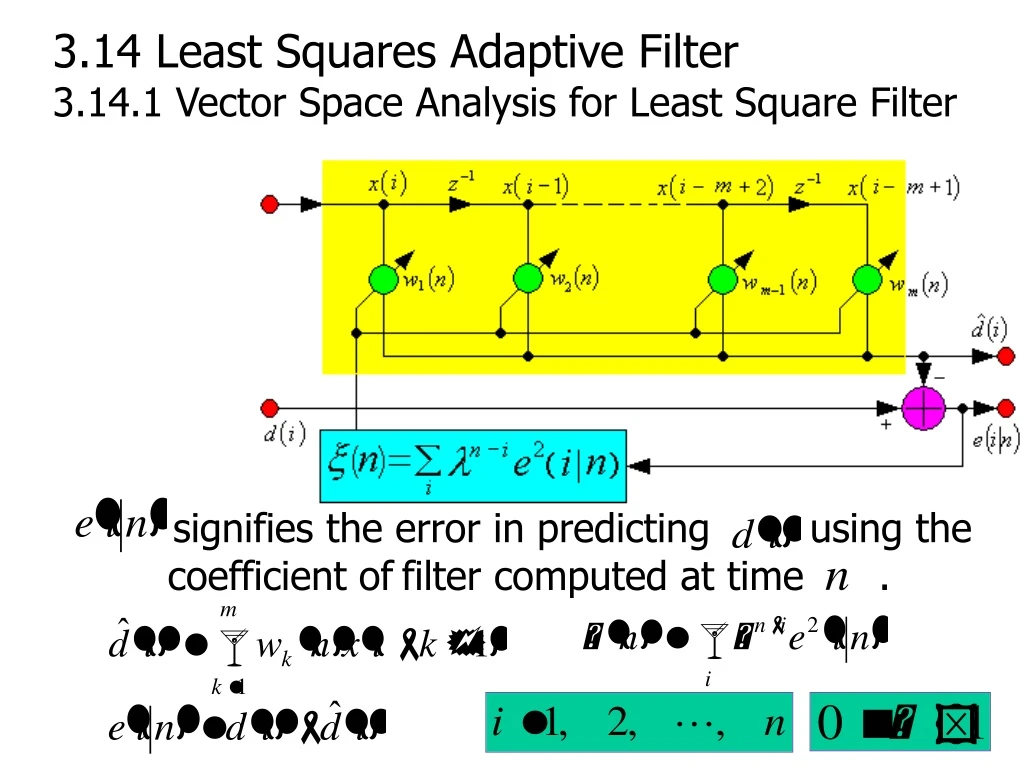
1. signifies the error in predicting using the coefficient offilter computed at time . 3.14 Least Squares Adaptive Filter 3.14.1 Vector Space Analysis for Least Square Filter

3. The Recursive Least Squares (RLS) Problem Finding the set of coefficients of the filter such that the cumulative error measure is minimized. prewindowed data

4. The vector and matrix representation for the RLS problem (1) The desired vector Example:

5. (2) The weight vector (3) The data matrix (prewindowed data)

6. (5) The error vector signifies the error in predicting using the coefficient offilter computed at time . (6) The vector and matrix representation

7. Although is very important in the application of RLS to nonstationary, it is often set equal to 1 if it is known that the data is stationary. A value of signifies that all data is equally weighted in the computation of , and this case often referred to as the prewindowed case. Progressively smaller values of compute based upon effectively smaller windows of data that are beneficial in nonstationary environments. For these reasons, is sometimes called the fade factor or forgetting factor for the filter. A value of in the range has proved to be effective in tracking local nonstationaries.

8. (7) The optimal weight vector of the LS Filter

9. (8) The LS estimation (the output of the LS filter)

10. (9) Vector Space Analysis for Least Square Filter The data vector The time-shifted vector The data vector space The dimension subspace spanned by the columns of .

11. Example

13. may be interpreted as a linear combination of the columns of .

14. The Least Squares (RLS) Problem (Summary) • Suppose column vectors of the data matrix • span a dimension subspace . • Find the vector in that closest to the • desired vector . The desired vector lies in the • dimension linear vector space. • Solution: • is the projection of onto the subspace • .

15. can be expressed by the linear combination • of the basis vectors of the subspace . • is closest to . The length of the error vector is the norm of the error vector. (4) The entire dimensional linear vector space containing may be defined as the direct sum of the two orthogonal subspaces

16. is the complement of the project of onto . is the orthogonal complement space of .

17. 3.14.2 Projection Matrix and Orthogonal Projection Matrix

18. Properties of Projection Matrix and Orthogonal Projection Matrix

19. Proving: supposed a discretionary vector v, and

20. The current data subspace is , which has the projection matrix and the orthogonal projection matrix . Suppose the additional vector is added to the set of the basis vectors of . The specific vector differs depending on the application. For example,

21. is the data subspace for an order least square filter. is the data subspace for an order least square filter.

22. In general, the vector will usually provide some information not contained in the basis vectors of . As the data subspace changes from to , then it is necessary to find the “new” projection matrices and in terms of the old projection matrices and . If this can be done in a recursive manner, then the groundwork will be laid for the fast RLS filter updates.

23. The vector itself cannot guaranteed to be orthogonal to . However, if may be used to create a vector that is orthogonal to , then the projection matrix ma be decomposed into

24. Proving formula 5

25. (6) Proving

26. (7)

27. Proving

28. By a judicious selection of and in properties (6),(7)(8), all time and order updates needed for both the LSL and transversal least squares filters may be derived.

29. 3.14.3 Time Update (1) Time Update of Projection Matrix Definition: The Unit Time Vector The projection matrix of

30. The orthogonal projection matrix of

33. Time Update of Projection Matrix

34. Appending the vector to the current data matrix provides a method for decomposing a projection matrix into its past and current components.

35. (2) The Angle Parameter Definition:

36. The relationship between and expressed by the angle parameter The property (6) of the projection matrix:

37. On the other hand:

38. 3.15 Least Square Lattice (LSL) Adaptive Algorithm Forward prediction

39. (prewindowed data) : LS forward prediction coefficients

40. The Forward Prediction Vector:

42. The Forward Prediction Error (FPE) Vector:

44. The current time FPE scalar sample: The benefit of writing ,as in the above equation, is that the FPE is now in the form required by the property (8) for the LS update of a scalar. This will be very important in the order updates for the LS lattice.

45. Backward prediction

46. The backward prediction vector:

47. The Backward Prediction Error Vector: The current time BPE scalar sample:

48. FPE and BPE Residuals:

49. 3.15.2 LS Lattice Structure of PE Filter The structure derived from the order update for FPE and BPE