Nonlinear Data-Based Reduced Models of Climate Variability
270 likes | 363 Views
Discover nonlinear data-based models capturing climate dynamics; empirical mode reduction, multi-level modeling, and illustrative QG3 model analysis presented.

Nonlinear Data-Based Reduced Models of Climate Variability
E N D
Presentation Transcript
Nonlinear, Data-based Reduced Models of Climate Variability Michael Ghil Ecole Normale Supérieure, Paris, and University of California, Los Angeles Joint work with Dmitri Kondrashov, UCLA; Sergey Kravtsov, U. Wisconsin–Milwaukee; Andrew Robertson, IRI, Columbia http://www.atmos.ucla.edu/tcd/
Motivation • Sometimes we have data but no models. • Linear inverse models (LIM) are good least-square fits to data, but don’t capture all the processes of interest. • Difficult to separate between the slow and fast dynamics (MTV). • We want models that are as simple as possible, but not any simpler. Criteria for a good data-derived model Fit the data, as well or better than LIM. Capture interesting dynamics: regimes, nonlinear oscillations. Intermediate-order deterministic dynamics. Good noise estimates.
Nonlinear dynamics: Discretized, quadratic: Multi-level modeling of red noise: Key ideas
Empirical mode reduction (EMR)–I • Multiple predictors: Construct the reduced model using J leading PCs of the field(s) of interest. • Response variables: one-step time differences of predictors; step = sampling interval = t. • Each response variable is fitted by an independent multi-level model: The main levell = 0 is polynomial in the predictors; all the other levels are linear.
Empirical mode reduct’n (EMR) – II • The number L of levels is such that each of the last-level residuals (for each channel corresponding to a given response variable) is “white” in time. • Spatial (cross-channel) correlations of the last-level residuals are retained in subsequent regression-model simulations. • The number J of PCs is chosen so as to optimize the model’s performance. • Regularization is used at the main (nonlinear) level of each channel.
Illustrative example: Triple well V (x1,x2) is not polynomial! • Our polynomial regression model produces a time series whose statistics are nearly identical to those of the full model!! • Optimal order is m = 3; regularization required for polynomial models of order m ≥ 5.
NH LFV in QG3 Model – I The QG3 model (Marshall and Molteni, JAS, 1993): • Global QG, T21, 3 levels, with topography; perpetual-winter forcing; ~1500 degrees of freedom. • Reasonably realistic NH climate and LFV: (i) multiple planetary-flow regimes; and (ii) low-frequency oscillations (submonthly-to-intraseasonal). • Extensively studied: A popular “numerical-laboratory” tool to test various ideas and techniques for NH LFV.
NH LFV in QG3 Model – II Output: daily streamfunction () fields ( 105 days) Regression model: 15 variables, 3 levels (L = 3), quadratic at the main level Variables: Leading PCs of the middle-level • No. of degrees of freedom = 45 (a factor of 40 less than in the QG3 model) • Number of regression coefficients P = (15+1+15•16/2+30+45)•15 = 3165 (<< 105) Regularization via PLS applied at the main level.
NH LFV in QG3 Model – IV The correlation between the QG3 map and the EMR model’s map exceeds 0.9 for each cluster centroid.
NH LFV in QG3 Model – V • Multi-channel SSA (M-SSA) identifies 2 oscillatory signals, with periods of 37 and 20 days. • Composite maps of these oscillations are computed by identifying 8 phase categories, according to M-SSA reconstruction.
NH LFV in QG3 Model – VI Composite 37-day cycle: QG3 and EMR results are virtually identical.
NH LFV in QG3 Model – VII Regimes vs. Oscillations: • Fraction of regime days as a function of oscillation phase. • Phase speed in the (RC vs. ∆RC) plane – both RC and ∆RC are normalized so that a linear, sinusoidal oscillation would have a constant phase speed.
NH LFV in QG3 Model – VIII Regimes vs. Oscillations: • Fraction of regime days: NAO– (squares), NAO+ (circles), AO+ (diamonds); AO– (triangles). Phase speed
NH LFV in QG3 Model – IX Regimes vs. Oscillations: • Regimes AO+, NAO– and NAO+ are associated with anomalous slow-down of the 37-day oscillation’s trajectory nonlinear mechanism. • AO– is a stand-alone regime, not associated with the 37- or 20-day oscillations.
NH LFV in QG3 Model – X Quasi-stationary states of the EMR model’s deterministic component. Tendency threshold • = 10–6; and • = 10–5.
NH LFV in QG3 Model – XI 37-day eigenmode of the regression model linearized about climatology* * Very similar to the composite 37-day oscillation.
NH LFV in QG3 Model – XII Panels (a)–(d): noise amplitude = 0.2, 0.4, 0.6, 1.0.
Conclusions on QG3 Model • Our ERM is based on 15 EOFs of the QG3 model and has L = 3 regression levels, i.e., a total of 45 predictors (*). • The ERM approximates the QG3 model’s major statistical features (PDFs, spectra, regimes, transition matrices, etc.) strikingly well. • The dynamical analysis of the reduced model identifies AO– as the model’s unique steady state. • The37-day mode is associated, in the reduced model, with the least-damped linear eigenmode. • The additive noise interactswith the nonlinear dynamics to yield the full ERM’s (and QG3’s) phase-space PDF. (*) An ERM model with 4*3 = 12 variables only does not work!
NH LFV – Observed Heights • 44 years of daily 700-mb-height winter data • 12-variable, 2-level model works OK, but dynamical operator has unstable directions: “sanity checks” required.
Concluding Remarks – I • The generalized least-squares approach is well suited to derive nonlinear, reduced models (EMR models) of geophysical data sets; regularization techniques such as PCR and PLS are important ingredients to make it work. • The multi-level structure is convenient to implement and provides a framework for dynamical interpretation in terms of the “eddy–mean flow” feedback (not shown). Easy add-ons, such as seasonal cycle (for ENSO, etc.). • The dynamic analysis of EMR models provides conceptual insight into the mechanisms of the observed statistics.
Concluding Remarks – II Possible pitfalls: • The EMR models are maps: need to have an idea about (time & space) scales in the system and sample accordingly. • Our EMRs are parametric: functional form is pre-specified, but it can be optimized within a given class of models. • Choice of predictors is subjective, to some extent, but their number can be optimized. • Quadratic invariants are not preserved (or guaranteed) – spurious nonlinear instabilities may arise.
References Kravtsov, S., D. Kondrashov, and M. Ghil, 2005: Multilevel regression modeling of nonlinear processes: Derivation and applications to climatic variability. J. Climate, 18, 4404–4424. Kondrashov, D., S. Kravtsov, A. W. Robertson, and M. Ghil, 2005: A hierarchy of data-based ENSO models. J. Climate, 18, 4425–4444. Kondrashov, D., S. Kravtsov, and M. Ghil, 2006: Empirical mode reduction in a model of extratropical low-frequency variability. J. Atmos. Sci., accepted. http://www.atmos.ucla.edu/tcd/
Nomenclature Response variables: Predictor variables: Each is normally distributed about Eachis known exactly. Parameter set {ap}: – known dependence of f on {x(n)} and {ap}. REGRESSION: Find
LIM extension #1 Do a least-square fit to a nonlinear function of the data: J response variables: Predictor variables (example – quadratic polynomial of J original predictors): Note: need to find many more regression coefficients than for LIM; in the example above P = J + J(J+1)/2 + 1 = O(J2).
Regularization • Caveat: If the number P of regression parameters is comparable to (i.e., it is not much smaller than) the number of data points, then the least-squares problem may become ill-posed and lead to unstable results (overfitting) ==> One needs to transform the predictor variables to regularize the regression procedure. • Regularization involves rotated predictor variables: the orthogonal transformation looks for an “optimal” linear combination of variables. • “Optimal” = (i) rotated predictors are nearly uncorrelated; and (ii) they are maximally correlated with the response. Canned packages available.
LIM extension #2 Motivation: Serial correlations in the residual. Main level, l = 0: Level l = 1: … and so on … Level L: rL– Gaussian random deviate with appropriate variance • If we suppress the dependence on x in levels l = 1, 2,… L, then the model above is formally identical to an ARMA model.