Download
1 / 35
350 likes | 484 Views
This presentation discusses the estimation of coefficients for nonlinear fluid-dynamic flows, particularly those governed by equations incorporating quadratic nonlinearity such as the Navier-Stokes equations. The focus is on leveraging observations from multivariate time series data to derive model parameters through advanced techniques like Principal Component Regression (PCR) and Partial Least Squares (PLS). The paper provides didactic examples including the Lorenz-63 model and multi-level regression frameworks, demonstrating the effectiveness of these approaches in capturing essential dynamics of complex systems.

E N D
Linear-Regression-based Models of Nonlinear Processes Sergey Kravtsov Department of Mathematical Sciences, University of Wisconsin-Milwaukee Collaborators: Dmitri Kondrashov, Andrew Robertson, Michael Ghil Presentation at March 2014
Motivation Many fluid-dynamical flows are governed, in discrete form, by equations with quadratic nonlinearity (e.g., Navier-Stokes): + NOISE where xi is a state vector (e.g., velocity field at a set of grid points), and a, b, c are constant coefficients Our task is to estimate a, b, c not from the first principles, but from observations of multivariate time series of xi We are looking at a subset of dynamical variables, and parameterize all others as noise
General Linear Least-Squares Minimize:
Regularization via SVD • Least-squares “solution” of is • “Principal Component” regularization:
Partial Least-Squares model selection • Involves rotated principal components (PCs), which are maximally correlated with response • Optimal number of rotated “latent” variables N is determined by cross-validation • Works best when combined with stepwise-regression- like model selection (editing out non-robust predictors via cross-validation: Kravtsov et al. 2011)
Lorenz-63 Example (cont’d) • Given short enough t, coefficients of the Lorenz model are reconstructed with a good accuracy for sample time series of length as short as T 1 • These coefficients define a model, whose long integration allows one to infer correct long-term statistics of the system, e.g., PDF Employing PCR and/or PLS regularization for short samples is advisable • Hereafter, we will always treat regression models as maps (discrete time), rather than flows (conti- nuous time).
Didactic Example–II (Triple well) V(x1,x2) is not polynomial • Polynomial regression model produces time series, whose statistics are nearly identical to those of the full model • Regularization required for polynomial models of order
Multi-level models (Kravtsov et al. 2005) Motivation: serial correlations in the residual Main (0) level: Level 1: … and so on … Level L: • rL– Gaussian random deviate with appropriate var. • If suppress dependence on x in levels 1–L, then the above model is formally identical to an ARMA model
Multi-level models – II • Multiple predictors: N leading PCs of the field(s) of interest (PCs of data matrix, not design matrix!) • Response variables: one-step [sampling interval] time differences of predictors • Each response variable is fit by an independent multi-level model. The main level is polynomial in predictors; all others – linear
Multi-level models – III • Number of levels L is such that each of the last-level residuals (for each channel corresponding to a given response variable) is “white” in time • Spatial (cross-channel) correlations of the last-level residuals are retained in subsequent regression-model simulations • Number of PCs (N) is chosen to optimize the model’s performance PLS/stepwise regression is used at the main (nonlinear) level of each channel
NH LFV in MM93 Model – I Model (Marshall and Molteni 1993): • Global QG, T21, 3-level with topography; perpetual-winter forcing; ~1500 degrees of freedom • Reasonably realistic in terms of LFV (multiple planetary-flow regimes and low-frequency [submonthly-to-intraseasonal] oscillations) • Extensively studied: A popular laboratory tool for testing out various statistical techniques
NH LFV in MM93 Model – II Output: daily streamfunction () fields ( 105 days) Regression model: 15 variables, 3 levels, quadratic at the main level Variables: Leading PCs of the middle-level • Degrees of freedom: 45 (a factor of 40 less than in the MM-93 model) • Number of regression coefficients: (15+1+15•16/2+30+45)•15=3165 (<< 105) PLS applied at the main level
Conclusions on MM93 Model • 15 (45)-variables regression model closely approximates 1500-variables model’s major statistical features (PDFs, spectra, regimes, transition matrices, and so on) Dynamical analysis of the reduced model was used to interpret its LFV (Kondrashov et al. 2006, 2010)
ENSO (Kondrashov et al. 2005) Data: • Monthly SSTs: 1950–2004, 30 S–60 N, 5x5 grid (Kaplan et al.) 1976/1977 shift removed SST data skewed: Nonlinearity important?
ENSO – II Regression model: • 2-level, 20-variable (EOFs of SST) • Seasonal variations in linear part of the main (quadratic) level • Competitive skill: Currently a member of a multi-model prediction scheme of the IRI (http://iri.columbia.edu/climate/ENSO/currentinfo/SST_table.html)
ENSO – III Observed • Quadratic model (100-member ensemble) • Linear model (100-member ensemble) Quadratic model has a slightly smaller rms error of extreme-event forecast (not shown)
ENSO – IV Spectra: Data Model SSA Wavelet QQ and QB oscillatory modes are reproduced by the model, thus leading to a skillful forecast
Conclusions on ENSO model Competitive skill; 2 levels really matter • “Linear,” as well as “nonlinear” phenomenology of ENSO is well captured • Statistical features related to model’s dynamical operator (Kondrashov et al. 2005)
Other applications of EMR modeling to date: Observed geopotential height modeling (Kravtsov et al. 2005) • Air–sea interaction over the Southern Ocean (Kravtsov et al. 2011) • EMR modeling of radiation belts (Kondrashov, Shprits, Ghil) Review in a book: Kravtsov et al. (2009), in Stochastic Physics and Climate modeling, T. Palmer & P. Williams, Eds., Cambridge University Press
CONCLUSIONS • General Linear Least-Squares is method well fit, in combination with regularization techniques such as PCR and PLS, for statistical modeling of geophysical data sets • Multi-level structure is convenient to implement and provides a framework for dynamical interpretation in terms of the “eddy – mean flow” feedback Easy add-ons, such as seasonal cycle • Analysis of regression models provides conceptual view for possible dynamical causes behind the observed statistics
CONCLUSIONS (cont’d) Pitfalls: • Models are maps: need to have an idea about (time) scales in the system and sample accordingly • Models are parameteric: functional form is pre-specified Choice of predictors is subjective • No quadratic invariants guaranteed – instability possible (work in progress)
New stuff: EMR model of NH U,V wind EMR-based model analyses thus far concentrated on large-scale low-frequency portion of the simulated variability How about empirical modeling valid throughout the whole spatiotemporal extent of variability scales? • Example: NCEP-1 daily U, V wind 1948–2008 Application: nudge a global climate model to the EMR-based climate surrogates to correct for biases, then do targeted regional downscaling with a nested dynamical model
EMR model details (850mb U, V) 1100 variables (PCs of combined U, V EOFs): >99% of variability captured • 3 levels, LINEAR MODEL at EACH level (good approximation – see next slide, can be modified) 4 separate models for each season (DJF, MAM, JJA, SON), seamless integration in time also developed: analogous models for 500 and 250mb fields, as well as combined 850, 500, 250-mb behavior
Performance in phys. space - I Daily simulated Daily observed
Performance in phys. space - II Daily observed 10-day LOW-PASS Daily simulated
Performance in phys. space - III Daily observed 8-day HIGH-PASS Daily simulated
Work in Progress advanced diagnostics of the linear EMR model: storm tracks etc. models for 850, 500, 250-mb U, V combined models with dependence on SST external predictors (e.g., Fig. on left) to match the design of CAM/WRF downscaling scheme synchronization of dynamical and empirical models (G. Duane, F. Selten and co-authors)