Innovative Spatial Modeling Approaches for Nonlinear Data Analysis
Explore cutting-edge methods for spatial data analysis with a focus on multinomial logit models, spatial autoregressive panel models, and spatial filtering techniques. Learn from experts in the field as they present their research on spatial maximum score estimation, urban accessibility indifference curves, and geographical efficiency measurements in panel data.


Innovative Spatial Modeling Approaches for Nonlinear Data Analysis
E N D
Presentation Transcript
Nonlinear Models with Spatial Data William Greene Stern School of Business, New York University Washington D.C. July 12, 2013
On Our Program School District Open Enrollment: A Spatial Multinomial Logit Approach; David Brasington, University of Cincinnati, USA, Alfonso Flores-Lagunes, State University of New York at Binghamton, USA, Ledia Guci, U.S. Bureau of Economic Analysis, USA Smoothed Spatial Maximum Score Estimation of Spatial Autoregressive Binary Choice Panel Models; Jinghua Lei, Tilburg University, The Netherlands Application of Eigenvector-based Spatial Filtering Approach to a Multinomial Logit Model for Land Use Data; Takahiro Yoshida & Morito Tsutsumi, University of Tsukuba, Japan Estimation of Urban Accessibility Indifference Curves by Generalized Ordered Models and Kriging; Abel Brasil, Office of Statistical and Criminal Analysis, Brazil, & Jose Raimundo Carvalho, Universidade Federal do Cear´a, Brazil Choice Set Formation: A Comparative Analysis, Mehran Fasihozaman Langerudi,Mahmoud Javanmardi, Kouros Mohammadian, P.S Sriraj, University of Illinois atChicago, USA, & Behnam Amini, Imam Khomeini International University, Iran Not including semiparametric and quantile based linear specifications
Also On Our Program Ecological fiscal incentives and spatial strategic interactions: the José Gustavo Féres Institute of Applied Economic Research (IPEA) Sébastien Marchand_ CERDI, University of Auvergne Alexandre Sauquet_ CERDI, University of Auvergne (Tobit) The Impact of Spatial Planning on Crime Incidence : Evidence from Koreai Hyun Joong Kimii Ph.D. Candidate, Program in Regional Information, Seoul National University & Hyung Baek Lim Professor, Dept. of Community Development SungKyul University (Spatially Autoregressive Probit) Spatial interactions in location decisions: Empirical evidence from a Bayesian Spatial Probit model Adriana Nikolic, Christoph Weiss, Department of Economics, Vienna University of Economics and Business A geographically weighted approach to measuring efficiency in panel data: The case of US saving banks Benjamin Tabak, Banco Central do Brasil, Brazil, Rogerio B. Miranda, Universidade Catolica de Brasılia, Brazil, & Dimas M Fazio, Universidade de Sao Paulo (Stochastic Frontier)
Spatial Autoregression in a Linear Model
Spatial Autocorrelation in Regression
Panel Data Applications (many at this meeting)
Analytical Environment Generalized linear regression Complicated disturbance covariance matrix Estimation platform: Generalized least squares, GMM or maximum likelihood. Central problem, estimation of
Practical Obstacles Numerical problem: Maximize logL involving sparse (I-W) Inaccuracies in determinant and inverse Appropriate asymptotic covariance matrices for estimators Estimation of . There is no natural residual based estimator Potentially very large N – GIS data on agriculture plots Complicated covariance structures – no simple transformations to Gauss-Markov form
Binary Outcome: Y=1[New Plant Located in County] Klier and McMillen: Clustering of Auto Supplier Plants in the United States. JBES, 2008
Outcomes in Nonlinear Settings Land use intensity in Austin, Texas – Discrete Ordered Intensity = ‘1’ < ‘2’ < ‘3’ < ‘4’ Land Usage Types, 1,2,3 … – Discrete Unordered Oak Tree Regeneration in Pennsylvania – Count Number = 0,1,2,… (Excess (vs. Poisson) zeros) Teenagers in the Bay area: physically active = 1 or physically inactive = 0 – Binary Pedestrian Injury Counts in Manhattan – Count Efficiency of Farms in West-Central Brazil – Stochastic Frontier Catch by Alaska trawlers - Nonrandom Sample
Nonlinear Outcomes Models Discrete revelation of choice indicates latent underlying preferences Binary choice between two alternatives Unordered choice among multiple choices Ordered choice revealing underlying strength of preferences Counts of events Stochastic frontier and efficiency Nonrandom sample selection
Modeling Discrete Outcomes “Dependent Variable” typically labels an outcome • No quantitative meaning • Conditional relationship to covariates No “regression” relationship in most cases. Models are often not conditional means. The “model” is usually a probability Nonlinear models – usually not estimated by any type of linear least squares Objective of estimation is usually partial effects, not coefficients.
Nonlinear Spatial Modeling Discrete outcome yit = 0, 1, …, J for some finite or infinite (count case) J. • i = 1,…,n • t = 1,…,T Covariates xit Conditional Probability (yit = j) = a function of xit.
Issues in Spatial Discete Choice A series of Issues Spatial dependence between alternatives: Nested logit Spatial dependence in the LPM: Solves some practical problems. A bad model Spatial probit and logit: Probit is generally more amenable to modeling Statistical mechanics: Social interactions – not practical Autologistic model: Spatial dependency between outcomes vs. utilities. Variants of autologistic: The model based on observed outcomes is incoherent (“self contradictory”) Endogenous spatial weights Spatial heterogeneity: Fixed and random effects. Not practical? The models discussed below
Two Platforms Random Utility for Preference Models Outcome reveals underlying utility • Binary: u* = ’x y = 1 if u* > 0 • Ordered: u* = ’x y = j if j-1 < u* < j • Unordered: u*(j) = ’xj , y = j if u*(j) > u*(k) Nonlinear Regression for Count Models Outcome is governed by a nonlinear regression • E[y|x] = g(,x)
Maximum Likelihood EstimationCross Section Case: Binary Outcome
Cross Section Case: n Observations
Spatially Correlated ObservationsCorrelation Based on Unobservables
Spatially Correlated ObservationsBased on Correlated Utilities
LogL for an Unrestricted BC Model
Spatial Autoregression Based on Observed Outcomes
See, also, Maddala (1983) From Klier and McMillen (2012)
Solution Approaches for Binary Choice Approximate the marginal density and use GMM (possibly with the EM algorithm) Distinguish between private and social shocks and use pseudo-ML Parameterize the spatial correlation and use copula methods Define neighborhoods – make W a sparse matrix and use pseudo-ML Others …
GMM in the Base Case with = 0 Pinske, J. and Slade, M., (1998) “Contracting in Space: An Application of Spatial Statistics to Discrete Choice Models,” Journal of Econometrics, 85, 1, 125-154. Pinkse, J. , Slade, M. and Shen, L (2006) “Dynamic Spatial Discrete Choice Using One Step GMM: An Application to Mine Operating Decisions”, Spatial Economic Analysis, 1: 1, 53 — 99. See, also, Bertschuk, I., and M. Lechner, 1998. “Convenient Estimators for the Panel Probit Model.” Journal of Econometrics, 87, 2, pp. 329–372
GMM in the Spatial Autocorrelation Model
Using the GMM Approach Spatial autocorrelation induces heteroscedasticity that is a function of Moment equations include the heteroscedasticity and an additional instrumental variable for identifying . LM test of = 0 is carried out under the null hypothesis that = 0. Application: Contract type in pricing for 118 Vancouver service stations.
An LM Type of Test? If = 0, g = 0 because Aii = 0 At the initial logit values, g = 0 If = 0, g = 0. Under the null hypothesis the entire score vector is identically zero. How to test = 0 using an LM test? Same problem shows up in RE models But, here, is in the interior of the parameter space!
Pseudo Maximum Likelihood Maximize a likelihood function that approximates the true one Produces consistent estimators of parameters How to obtain standard errors? Asymptotic normality? Conditions for CLT are more difficult to establish.
Pseudo MLE
Covariance Matrix for Pseudo-MLE
‘Pseudo’ Maximum Likelihood Smirnov, A., “Modeling Spatial Discrete Choice,” Regional Science and Urban Economics, 40, 2010.
Pseudo Maximum Likelihood Bases correlation on underlying utilities Assumes away the correlation in the reduced form Makes a behavioral assumption Still requires inversion of (I-W) Computation of (I-W) is part of the optimization process - is estimated with . Does not require multidimensional integration (for a logit model, requires no integration)
Other Approaches Case A (1992) Neighborhood influence and technological change. Economics 22:491–508 Beron KJ, Vijverberg WPM (2004) Probit in a spatial context: a monte carlo analysis. In: Anselin L, Florax RJGM, Rey SJ (eds) Advances in spatial econometrics: methodology, tools and applications. Springer, Berlin Beron and Vijverberg (2003): Brute force integration using GHK simulator in a probit model. Impractical. Case (1992): Define “regions” or neighborhoods. No correlation across regions. Produces essentially a panel data probit model. (Also Wang et al. (2013)) LeSage: Bayesian - MCMC Copula method. Closed form. See Bhat and Sener, 2009.
See also Arbia, G., “Pairwise Likelihood Inference for Spatial Regressions Estimated on Very Large Data Sets” Manuscript, Catholic University del Sacro Cuore, Rome, 2012.
Partial MLE (Looks Like Case, 1992)
Bivariate Probit Pseudo MLE Consistent Asymptotically normal? • Resembles time series case • Correlation need not fade with ‘distance’ Better than Pinske/Slade Univariate Probit? How to choose the pairings?
LeSage Methods - MCMC • Bayesian MCMC for all unknown parameters • Data augmentation for unobserved y* • Quirks about sampler for rho.
An Ordered Choice Model (OCM)
OCM for Land Use Intensity
A Dynamic Spatial Ordered Choice Model Wang, C. and Kockelman, K., (2009) Bayesian Inference for Ordered Response Data with a Dynamic Spatial Ordered Probit Model, Working Paper, Department of Civil and Environmental Engineering, Bucknell University.