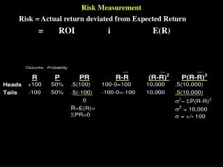
Risk Measurement
230 likes | 254 Views
Risk Measurement. Index. Risk Management Framework Risk Measurement Risk Attribution Risk Budgeting Risk Measures Volatility and Tracking Error (TE) Duration Shortfall probability Largest loss with given probability (VaR) Expected size of shortfall (C-VaR) Details on Volatility

Risk Measurement
E N D
Presentation Transcript
Index • Risk Management Framework • Risk Measurement • Risk Attribution • Risk Budgeting • Risk Measures • Volatility and Tracking Error (TE) • Duration • Shortfall probability • Largest loss with given probability (VaR) • Expected size of shortfall (C-VaR) • Details on Volatility • Details on Monte Carlo Simulation
I. Risk Management Framework • Risk Measurement: What is our risk? How do we measure it? • Risk Attribution: Where does our risk come from? What are the factors contributing to risk? • Risk Allocation: How do we allocate risk going forward?
II. Measures of Risk • Volatility and Tracking Error (TE) • Duration • Shortfall probability • Largest loss with given probability (VaR) • Expected size of shortfall (C-VaR)
II. Measures of Risk • Overview of some Market Risk Measures Expected Return Value at Risk, p% Volatility Conditional VaR
II. Measures of Risk 1. Volatility & Tracking Error • Volatility is the square root of the variance; where variance measures the dispersion of individual observations around their mean
II. Measures of Risk 1. Volatility & Tracking Error • TE is the standard deviation of the excess returns relative to a certain benchmark (i.e. the standard deviation of alphas)
II. Measures of Risk 2. Duration: • Modified Duration : Duration measures the percentage change in the bond price for 100 basis point change in rates • First derivative of the pricing function
II. Measures of Risk 2. Modified Duration: Calculation 5 Year; 10% Coupon; Yield 8%; Price 107.98 Macaulay Duration: weighted average maturity of a security's cash flows, where the present values of the cash flows serve as the weights Modified Duration = Macaulay Duration/(1+(yield/k)) = 4.204/(1+8%) =3.89
II. Measures of Risk 2. Modified Duration Calculation: The Concept of DV01: • DV01 is a (very) slight variation on the previous idea of modified duration. • Gives the market value (in units of currency) of change portfolio value associated with a one basis point change in yields.
II. Measures of Risk 3. Shortfall Probability • The probability that portfolio return falls below a certain threshold level on a specified time-horizon • Widely used measure: Probability of Negative Return
II. Measures of Risk 4. Value at Risk • It estimates the maximum amount that you are expected to lose over a specified time horizon at a specified confidence level of 5. Conditional Value at Risk • Expected loss, if the loss is larger than the VaR
Risk: different perspectives • Asset-only : Regard portfolio on a stand-alone basis • Asset vs. Liabilities
III. Estimating Volatility 1. Traditional measure of volatility for the calculation of a continuously compounded return over successive days • The mean return of these individual returns is calculated as:
III. Estimating Volatility 2.Weighting Scheme: • The simple approach of calculating volatility weigh each observation equally. • If the goal is to estimate the current level of volatility , we may want to weigh recent data more heavily. • The weights must sum to 1 and if the objective is to generate a greater influence on recent observations, then the α’s will decline in value for older observation.
III. Estimating Volatility 3.Extension to Weighting scheme: Autoregressive Conditional Heteroskedastic model ARCH(m) • One extension to this weighting scheme is to assume a long-run variance level in addition to the weighted squared return observations. • The most frequently used model is an Autoregressive Conditional Heteroskedastic model ARCH(m) which can be represented by;
III. Estimating Volatility 4. Exponentially Weighted moving average model (EWMA) • It is a specific case of the general weighting model presented before. • The main difference is that the weights are assumed to decline exponentially back through time. • Interpretation: the day-n volatility estimate is calculated as a function of the volatility calculated as of day n-1 and the most recent squared return. Depending on the weighting term λ which ranges between 0 and 1, the previous volatility and most recent squared returns will have different returns.
III. Estimating Volatility 4. Exponentially Weighted moving average model (EWMA): • Example: The decay factor in an exponentially weighted moving average model is estimated to be 0.94 for daily data. Daily volatility is estimated to be 1% and today’s stock market return is 2%. What is the estimate of volatility using the EWMA model? σn2 = 0.94 * 0.012 + (1 - 0.94) * 0.02 2 σn =√0.000118 = 1.086% • One benefit of the EWMA is that it requires few data points. Specifically all we need to calculate the variance is the current estimate of the variance and the most recent squared return. The current estimate of variance will then feed into the next period’s estimate, as will the period’s squared return.
III. Estimating Volatility 5. Generalized Autoregressive Conditional Heteroskedastic model: GARCH(m) • Prior to GARCH there was EWMA which has been superseded by GARCH. • EWMA is a special case of the a GARCH (1,1) volatility process with α0 = 0, α = 1-λ and ß = λ
III. Estimating Volatility 5. Generalized Autoregressive Conditional Heteroskedastic model: GARCH(m) • Example: GARCH(1,1) • The parameters of a generalized autoregressive conditional heteroskedastic GARCH(1,1) model are α0 = 0.000003, α = 0.04 and ß = 0.92. if daily volatility is estimated to be 1% and today’s stock market return is 2% what is the new estimate of volatility using the GARCH(1,1) model ? σn2 = 0.000003 +0.04 * 0.022 + 0.92* 0.012 = 0.000111 σn =√0.000111 = 1.054%
III. Estimating Volatility Estimation and Performance of GARCH models: • One of the very useful features of GARCH models is that they do a very good job at modeling volatility clustering. • GARCH models do a good job too in forecasting volatility from a volatility term structure perspective. GARCH-generated volatility does an excellent job in predicting how the volatility term structure responds to changes in volatility. • This modeling tool is quite frequently used by financial institutions when estimating exposure to various option positions.