Download
1 / 26
260 likes | 388 Views
This presentation discusses methods for spatial searching, indexing, and mapping species-level distribution data. Key aspects include approaches to coding for spatial searches, user-defined search areas, and different mapping options. Specific examples from the OBIS and CAAB databases illustrate the application of techniques such as grid squares and c-squares for indexing and mapping. The talk also covers various mapping software options, considering their performance, ease of use, cost, and compatibility with existing systems.

E N D
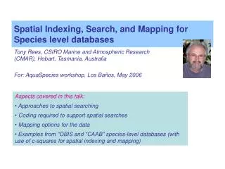
Spatial Indexing, Search, and Mapping for Species level databases Tony Rees, CSIRO Marine and Atmospheric Research (CMAR), Hobart, Tasmania, Australia For: AquaSpecies workshop, Los Baños, May 2006 • Aspects covered in this talk: • Approaches to spatial searching • Coding required to support spatial searches • Mapping options for the data • Examples from “OBIS and “CAAB” species-level databases (with use of c-squares for spatial indexing and mapping)
(1) Typical species-level distribution data – example from OBIS • (Typically patchy / incomplete, however will not worry about this now) • What search method(s) to offer? e.g... • named region, e.g. country name/EEZ • grid square or squares • user defined area (e.g. bounding box, point + radius, polygon...) • What should be returned in first instance? i.e... • build species list for the search region – maybe filtered by category, or • all the point data – maybe filtered as above
(2) Search by named region • Possible approaches: • Put everything in a GIS, search against named region’s polygon at run time • Classify every point with its relevant region name/s in advance, store with the point data • Classify every species with its relevant (unique) region name/s in advance, store in a new table (as “species-level metadata”)
(3) Search by grid square – example from OBIS Australia site(could also show the squares on the graphic, as per inset)
Search by grid square • Available options: • Fixed Size Grid Squares • Variable Size Grid Squares (nested squares) • Local or global grid? • Constant dimensions in degrees or km? • Possible approaches: • Classify every point with its relevant square ID/s in advance, store with the point data • Classify every species with its relevant (unique) square ID/s in advance, store in a new table (as “species-level metadata”)
“Data level index” example – 1 code (c-square) for every data point
“Metadata level index” example – 1 row (multiple squares) per species ID (NB, could also disaggregate this to a many:many table if preferred)
(4) Search by user-defined area • Available approaches: • Bounding box – enter coordinates, drag a rectangle in a java applet, or select from a list • (most common method) • Point + radius (normally expressed in distance e.g. km, miles) • (less common, but may match some user expectations; harder to implement) • User-defined polygon • (hard to implement in web environment, potentially slow) • ... all implemented against latitude/longitude values stored with the data.
(5) Mapping software • Possible approaches: • Deploy commercial software in-house (e.g.: ArcIMS) • Deploy free / open source software in-house (e.g.: MapServer, c-squares mapper) • Construct own mapper and deploy • Send data / squares to remote utility (third party mapper), e.g.: • BeBIF, CBIF Mappers • KGS Mapper (Kansas), ACON Mapper (Canada) • C-squares Mapper (Australia) • Google Earth (requires client on user’s PC)
Some aspects to consider... • Features offeredvs. anticipated requirements • Cost(including indirect costs e.g. person time / complexity to deploy, hardware requirements, ongoing admin / maintenance needs, also ongoing fees if any) • System Architecture, e.g. local vs. remote hosting, OGC compliant WMS plus client vs. self-contained system, etc. • Performance(speed of rendering e.g. 200, 2000, 20000, 200000 points; ultimate limit; bandwidth constraints if applicable) • Map quality, range of options available(including projections, map size / quality, variety of base maps, available scales, control of symbology / legends, etc.) • Useability(interface design and ease of use, browser / client machine needs) • Support (where from, what cost, responsiveness, what dedicated resources / guarantees) • Reliability (including system release status, possible points of failure, redundancy / risk management) • Compatibility with existing / future project, agency, community practices • Extensibility to cope with present and future needs (how, who can do it, what process / timelines available, source code available or not, programming language, etc.) Choosing Mapping software
Basic • Map data points on one or multiple base maps • Basic zoom and pan • Intermediate • Plot multiple data sets (e.g. different species, data sources, time periods), colour coded as necessary • Show data that cross the date line / poles as uninterrupted views • More sophisticated / detailed zoom and pan, improved map quality • Add / remove layers for display • Render line, polygon data • Degree of symbology control, labelling, legends, etc. • “Click on map” functionality to query underlying data • Advanced • Full range of projections available • Ingest external base data layers as images via WMS • Export species data layers as images via WMS • Calculate data statistics, summaries on-the-fly • Full symbology and layer transparency control Possible mapper features...
A few benchmarks ... from OBIS-SEAMAP (2006) report comparing MapServer, ArcIMS, and Google Earth Performance: Development programming:
Museum Victoria Species Mapper – Blue Whale (example of freeware “fly” mapper with local customisation)
BeBIF Point Data Mapper – Hoplostethus atlanticus (via GBIF) – 10,000 records
CMAR C-squares Mapper – Hoplostethus atlanticus (via OBIS) – 566 squares (representing 10,000 records)
C-squares Mapper – Predicted distribution of Xiphias gladius (via AquaMaps) – 85,000 squares in 5 colour codes (=probability classes)
ACON Mapper – Hoplostethus atlanticus (via OBIS) – includes statistics, on-the-fly binning, sort by data provider, etc.
True web GIS – Blue Whale data points + on-the-fly user-selectable layers, e.g. SST data (OBIS-SEAMAP site using MapServer)
(7) Example “CAAB” species name search result (NB, each species name is associated with stored list of 0.1 degree squares in this database) • Clicking on the map triggers a spatial query to the underlying base data table.
URLs mentioned in text: • AquaMaps: FishBase > tools > AquaMaps (uses c-squares mapper) • CAAB: http://www.marine.csiro.au/caab/ • C-squares: http://www.marine.csiro.au/csquares/ • FishBase: http://www.fishbase.org/ • GBIF: http://www.gbif.org/ (includes links to BeBIF, CBIF mappers) • Google Earth: http://earth.google.com/ • Museum Victoria Bioinformatics: http://www.museum.vic.gov.au/bioinformatics/ > mammals > map searches • OBIS: http://www.iobis.org (includes links to c-squares, ACON, KGS mappers) • OBIS Australia: http://www.obis.org.au/ • OBIS-SEAMAP: http://seamap.env.duke.edu/ (MapServer based site)
Overview of the c-squareshierarchical grid square notation (refer www.marine.csiro/csquares/ for more information) • C-squares principle • The world is first divided into 10x10 degree squares (global total: 648) • example code: 3414 • Each 10x10 degree square is divided into 4 5x5 degree squares (total: 2,592) • example code: 3414:1 • Each 5x5 degree square is divided into 25 1x1 degree squares (total: 64,800) • example code: 3414:132 • Each 1x1 degree square is divided into 4 0.5x0.5 degree squares (total: 259,200) • example code: 3414:132:3 • (etc.). NB, can then search at any higher level of the hierarchy, as required, since all nested parent codes are included as initial portion of the “child” code. • A simple algorithm will encode lat/lon to c-squares code, and vice versa. • Choice of resolution for encoding • Half degree squares (50 km nominal resolution) seems to be good compromise between spatial resolution and index size for global datasets (0.1x0.1 degrees may be preferred for regional scale use).
Actual size of half degree squares (e.g. cf. UK). NB, if data are encoded at this resolution, can then be queried at one, five or ten degree square sizes as well. 0.5 degree squares measure approximately 55 x 35 km at this latitude.