Download
1 / 36
380 likes | 829 Views
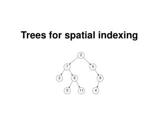
Trees for spatial indexing. Tree (data structure) . Introduction B-Tree,B+-Tree,B*-Tree Spatial Access Method (SAM) vs Point Access Method (PAM) Buddy-Tree, UB-Tree (8 slides) R-Tree X-Tree, TV-Tree. Pantheon Problem. 200’000’000 points are in a database.

E N D
Tree (data structure) • Introduction • B-Tree,B+-Tree,B*-Tree • Spatial Access Method (SAM)vsPoint Access Method (PAM) • Buddy-Tree, UB-Tree (8 slides) • R-Tree • X-Tree, TV-Tree
Pantheon Problem • 200’000’000 points are in a database. • Indexing in a B-Tree is not suffisant. We want to optimize the query range. • Which indexing method should we use ? • What is the best structure ?
What kind of data structure ? Structur depends on what kind of data : • point access method : A data structure to search for lines, polygons, … etc. • k-d tree • quadtree • UB-tree • buddy tree • Spatial access method : A data structure and associated algorithms primarily to search for points defined in multidimensional space. • D-tree • P-tree • R+-tree • R-tree • R*-tree
Types of queries in spatial data 'geometry' refers to a point, line, box or other two or three dimensional shape, the kind of queries we need are : • Distance(geometry, geometry) • Equals(geometry, geometry) • Disjoint(geometry, geometry) • Intersects(geometry, geometry) • Touches(geometry, geometry) • Crosses(geometry, geometry) • Overlaps(geometry, geometry) • Contains(geometry, geometry) • Intersects(geometry, geometry) • Several other operations performed on only one geometry such as length, area and centroid
Introduction • Some Definitions : • Node : A node may contain a value or a condition or represent a separate data structure or a tree of its own. Each node in a tree has 0 or more child nodes. A node that has a child is called the child's parent node (or ancestor node, or superior). A node has at most one parent. • Root nodes : The topmost node in a tree is called the root node. Being the topmost node, the root node will not have parents. Every node in a tree can be seen as the root node of the subtree rooted at that node. • Leaf nodes : Nodes at the bottom most level of the tree are called Leaf nodes. Since they are at the bottom most level, they will not have any children.
Tree of the trees B-Tree … … … … B+ B* … R-Tree … Buddy UB-Tree … R*-Tree UBU X TV ? ? Spatial Access Method (SAM)vsPoint Access Method (PAM)
Common Operations • Enumerating all the items • Searching for an item • Adding a new item at a certain position on the tree • Deleting an item • Removing a whole section of a tree (called pruning) • Adding a whole section to a tree (called grafting) • Finding the root for any node
B-Tree • a B-tree is a tree data structure that keeps data sorted and allows insertions and deletions in logarithmic amortized time. It is most commonly used in databases and filesystems. • in a 2-3 B-tree (often simply 2-3 tree), each internal node may have only 2 or 3 child nodes. • Each internal node's elements act as separation values which divide its subtrees.
B+-Tree • A B+ tree is a variation on a B-tree. In a B+ tree, in contrast to a B-tree, all data is saved in the leaves. Internal nodes contain only keys and tree pointers. All leaves are at the same lowest level. Leaf nodes are also linked together as a linked list to make range queries easy.
R-Tree • Extends the B+-Tree • All non-leaf node contains entries of form (cp,rectangle) where cp is the address of a child node and rectangle is the minimum bounding box rectangle (MBR). • ~ Leaf nodes contain entries of the form (dataObject,Rectangle). • We use the term directory rectangle which is the MBR of the underlying rectangles.
R-Tree properties • Let M be the maximum number of entries that fit in one node and let m be a parameter specifying the minimum number of entries in a node (2 ≤ m ≤ M), an R-Tree statisfies the following properties • The root has at least two children unless it’s a leaf. • Every non-leaf node has beetween m and M children unless it’s a root. • Every leaf node contains beetween m and M entries unless it’s a root. • All leaves appear on the same level.
PAM’s • The basic principle of all multidimensional PAMs is to partition the data space into page regions. We classify PAMs according to 3 properties :
Buddy-Tree • The Buddy-Tree uses similar concepts as the R-Tree. • But it is extended and has more interesting properties : • It does not partition empty space • Insertion and deletion of a record is restricted to exactly one path. • It does not allow overlap in the directory nodes.
Buddy-Tree : Formal Definition • The nodes of the tree-directory consist of a collection of entries {E1,…,Ek}, k ≥ 2. • Each entry Ei, 1 ≤ i ≤ k, is given by a tuple Ei=(Ri,pi) where Ri is a d-dimensional rectangle and pi is a pointer referring to as subtree or to a data page containing all the records of the file which are in the rectangle Ri. • The set of rectangles in a directory node must be a regular B-partition
B-Rectangle, B-partition • Given 2 d-dimensional rectangles R,S with R ≤ S, R is called a B-rectangleof S iff it can be generated by successive halfing of S. • A B-regionof R, written B(R) is the smallest rectangle such that R ≤ B. • Such a B-region also exists for a union of rectangles R1 U R2 U … U Rk, k ≥ 1. • A set of d-dimensional rectangles {R1,…,Rk}, k ≥ 1, is called a B-partition of the data space D, iff B(Ri) ∩ B(Rj) = Ø
The Buddies • Let V = {R1,…,Rk} a B-partition, k > 1, and let S,T Є V, S ≠T. • The rectangles S,T are called buddies iff B(S U T) ∩ B(R) = Ø For all R Є V\{S,T} S S T T S,T are Buddies S,T are NOT Buddies
Dynamic behavior • To obtain an efficient dynamic behavior it must be possible to merge without destroying the order preservation. • For this the regions of the pages must be buddies. • In the buddy-tree the set of rectangles in a directory node must be a regular B-partition. • We say that a B-parition is regular iff all B-rectangles B(Ri) 1 ≤ i ≤ k can be represented in a kd-trie. • A kd-trie is a binary tree where the internal ndoes consist of an axis and 2 pointers referring to subtrees.
Example • Here we say a regular B-Partition because we can represent it by a kd-trie t1 t3 t1 t2 s t3 s t2 B-Partition Kd-trie
UB-Tree (Universal B-Tree) • Methods with good performance are guaranted for only 1 dimension. UB-Tree can handle multidimensional data. • We can implement the UB-Tree on top of any database system. ( by preprocessing techniques )
UB-Tree (Universal B-Tree)[2] • Basic Concepts • Area : First we Partition a cube C of dimension n into 2n subcubes numbered : sc(i) for i=1,2,…,2n. • For example : in 2 dimensions. Sc(1) Sc(2) Sc(3) Sc(4) • AreaC(k) := Ui=1 to k, sc(i) for k = 0,1,…,2n • AreaC(k.j) := AreaC(k) U Areasc(k+1)(J) Area(3)
Concept of Address An addressα is a sequence I1,i2,… il where ijЄ 0,1,… 2n For example this area has address 0.3, noted alpha(A) = 0.3
Definitions and lemmas • Region : is the difference of 2 areas. • Address of pixel : is the address of the area defined by including the pixel as the last and smallest subcube contained in this Area. • There is a one-to-one map beetween Cartesian coordinates (x1,x2,…,xn) of a n-dimensional pixel and its address α. • Alpha(cart(α)) = α
Definitions and lemmas[2] • A point (x1,x2,…xn) has address region(β,δ), Γ =alpha(x1,x2,…,xn), it belong to the unique region(β,δ) with the condition β< Γ. region(0.1,3)
Range Queries • The query is defined by an interval for each dimension. Each dimension can be beetween (-∞,+∞). • The query is the cartesian product of the intervals for all dimensions, called the query box.
Range queries (2) • Definition : we call all subcubes of level s of a cube brothers. • Those with a smaller address are younger and those with a larger are older.
Complexity of UB-Tree • N is the number of objects, k = 1/2M. Let Q be the number of objects intersecting the querybox q. Let r be the number of regions intersecting q. • Point-Query : O(logk(N)) • Range Query : r * O(logk(N)), For points only it’s : (N*Q/M) * O(logk(N)) • Point insertion : O(logk(N))
Spatial Access Method • Spatial indexes are used by spatial databases to optimize spatial queries. Indexes used by non-spatial databases cannot effectively handle features such as how far two points differ and whether points fall within a spatial area of interest. • TV-Tree • X-Tree
TV-Tree (Telescopic-Vector tree) • The basis of the tv-tree is to use dynamically contracting and extending feature vectors. ( Like in classification )
TV-tree • We have also a hierarchical structure: • The objects are clustered into leaf nodes of the tree, and the (MBR), minimum bounding region is stored in the parent node. • Parents are recursively grouped, until the root is formed. • At the top levels it’s optimal because it uses only a few basic features.
TV-tree • The TV-tree can be applied to a tree with nodes that describe bounding regions of any shape (cubes,spheres,rectangles, … etc ).
Telescoping function • The telescoping problem can be described as follows. • Given an n x 1 feature vector x and m x n (m≤n) contraction matrix Am. • The Amx is an m-contraction of x. • A sequence of such matrices Am with m=1,… describes a telescoping function provided that the following condition is satisfied : If the m1-contractions of the 2 vectors x and y are equal, then so are their respective m2-contractions, for every m2 ≤ m1.
Multiple shapes • We can use for example a sphere, because it’s only a center and a radius r. Represents the set of points with euclidean distance ≤ r. • ~the euclidean distance is a special case of the Lp metrics with p=2. • For L1 metric (manhattan distance) it defines a diamond shape. • The TV-tree is working with any Lp-sphere.
TMBR (Telescopic Minimum Bounding Region) • Each node in the TV-Tree represents the MBR (an Lp-sphere) of all its descendents. • Each region is represented by a center, which is a vector determined by the telescoping vectors representing the objects and a scalar radius. • We use the term TMBR to denote an MBR with such a telescopic vector as a center.