Download
1 / 23
240 likes | 410 Views
Spatial Autocorrelation Basics NR 245 Austin Troy University of Vermont. SA basics. Lack of independence for nearby obs Negative vs. positive vs. random Induced vs inherent spatial autocorrelation First order (gradient) vs. second order (patchiness) Within patch vs between patch

E N D
Spatial Autocorrelation BasicsNR 245Austin TroyUniversity of Vermont
SA basics • Lack of independence for nearby obs • Negative vs. positive vs. random • Induced vs inherent spatial autocorrelation • First order (gradient) vs. second order (patchiness) • Within patch vs between patch • Directional patterns: anisotropy • Measured based on point pairs
Spatial lags Source: ESRI, ArcGIS help
Statistical ramifications • Spatial version of redundancy/ pseudo-replication • OLS estimator biased and confidence intervals too narrow. • fewer number of independent observations than degrees of freedom indicate • Estimate of the standard errors will be too low. Type 1 errors • Systematic bias towards variables that are correlated in space
Tests • Null hypothesis: observed spatial pattern of values is equally likely as any other spatial pattern • Test if values observed at a location do not depend on values observed at neighboring locations
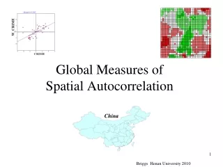
Moran’s I • Ratio of two expressions: similarity of pairs adjusted for number of items, over variance • Similarity based on difference from global mean See http://www.spatialanalysisonline.com/output/html/MoranIandGearyC.html#_ref177275168 for more detail
Moran’s I Where N is the number of casesXi is the variable value at a particular locationXj is the variable value at another location is the mean of the variableWij is a weight applied to the comparison between location i and location j See http://www.spatialanalysisonline.com/output/html/MoranIandGearyC.html#_ref177275168 for more detail
Moran’s I Deviation from global mean for j • Wij is a contiguity matrix. Can be: • Adjacency based • Inverse distance-based (1/dij) • Or can use both # of connections In matrix See http://www.spatialanalysisonline.com/output/html/MoranIandGearyC.html#_ref177275168 for more detail
Moran’s I “Cross product”: deviations from mean of all neighboring features, multiplied together and summed When values of pair are either both larger than mean or both smaller, cross-product positive. When one is smaller than the mean and other larger than mean, the cross-product negative. The larger the deviation from the mean, the larger the cross-product result. See http://www.spatialanalysisonline.com/output/html/MoranIandGearyC.html#_ref177275168 for more detail
Moran’s I • Varies between –1.0 and + 1.0 • When autocorrelation is high, the coefficient is high • A high I value indicates positive autocorrelation • Zero indicates negative and positive cross products balance each other out, so no correlation • Significance tested with Z statistic • Z scores are standard deviations from normal dist Source: ESRI ArcGIS help
Geary’s C • One prob with Moran’s I is that it’s based on global averages so easily biased by skewed distribution with outliers. • Geary’s C deals with this because: • Interaction is not the cross-product of the deviations from the mean like Moran, but the deviations in intensities of each observation location with one another
Geary’s C • Value typically range between 0 and 2 • C=1: spatial randomness • C< 1: positive SA • C>1: negative SA • Inversely related to Moran’s I • Emphasizes diff in values between pairs of observations, rather than the covariation between the pairs. • Moran more global indicator, whereas the Geary coefficient is more sensitive to differences in small neighborhoods.
Scale effects • Can measure I or C at different spatial lags to see scale dependency with spatial correlogram Source:http://iussp2005.princeton.edu/download.aspx?submissionId=51529
LISA • Local version of Moran: maps individual covariance components of global Moran • Require some adjustment: standardize row total in weight matrix (number of neighbors) to sum to 1—allows for weighted averaging of neighbors’ influence • Also use n-1 instead of n as multiplier • Usually standardized with z-scores • +/- 1.96 is usually a critical threshold value for Z • Displays HH vs LL vs HL vs LH And expected value where
Local Getis-OrdStatistic (High/low Clustering) • Indicates both clustering and whether clustered values are high or low • Appropriate when fairly even distribution of values and looking for spatial spikes of high values. When both the high and low values spike, they tend to cancel each other out • For a chosen critical distance d, where xi is the value of ith point, w(d) is the weight for point i and j for distance d. Only difference between numerator and denominator is weighting. Hence, w/ binary weights, range is from 0 to 1.
Local Moran: inverse distance + 2000 m threshold