Download
1 / 27
270 likes | 456 Views
STAT131 Week 5 Lecture1a Formalising the Introduction to Discrete Random Variables. Anne Porter alp@uow.edu.au. Review. The game Beat the Butcher was used to introduce a topic - modelling variation in data This lecture will introduce a number of formal definitions and notation

E N D
STAT131Week 5 Lecture1a Formalising the Introduction to Discrete Random Variables Anne Porter alp@uow.edu.au
Review • The game Beat the Butcher was used to introduce a topic - modelling variation in data • This lecture will introduce a number of formal definitions and notation • This lecture will formalise that game as we examine the topic of Random Variables • And move on to examine the Binomial model
Definitions: Random Variable X A Random Variable X is a function, often denoted • f(x) , px, or P(X=x) • It is defined by • a set of numerical outcomes x • AND • the set of probabilities that describe them
P(X=x) • The probability that the random variable big X takes on the value little x. What does this P(X=x) mean?
Sample of data What happens as relative frequency becomes very large? The probability of that event can be defined as the limit of the relative frequency Each repetition provides a single numerical value (an outcome) and the resulting values ne are simple random sample of experiments
Sample of data Is 100 large?
Sample of data Is 100 large? Not really! But we will use it to demonstrate
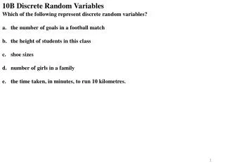
Example: What was the variable of interest in playing beat the butcher? ...the random variable, 'number of items before the gong' when playing beat the butcher. What values did X take on? 3,4,……, 11 Another example might be: the number of girls in families with three children.
To be a probability distribution of a discrete distribution • all P(X=x) > 0 and all P(X=x) < =1 • and SP(X=x)=1 • OR in the alternative notation • all px > 0 and all px < 1 • and Spx=1
Defining a probability distribution Two methods of defining • Charts showing x and P(X=x) • Tables showing x and P(X=x)
Defining a probability distribution: bar charts 3 4 5 6 7 8 9 10 11
Features of interest forDiscrete Random Variables • P(X=x)? (May involve reading table or calculations) • Centre • Mean • Spread • Variance • Standard Deviation • Do the data fit a given model?
Answering probability questions What is the probability that the gong will occur after the 8th item is read? 0.20 What is the probability That the gong will occur after 8 or more items are read? 0.64
Answering questions What is the probability that the number of items will be less than 8 before the gong?
Answering questions What is the probability that the number of items will be less than 8 before the gong? 1- 0.64=0.36 Or 0.02+0.06+0.06+0.08+0.14=0.36
Centre: E(X) or mean of model mx or x.P(X=x)
Centre: E(X) or mean of model mx or x.P(X=x) x.P(X=x) 3x0.02 4x0.06 5x0.06 6x0.08 7x0.14 8x0.20 9x0.28 10x0.10 11x0.06 0.06 0.24 0.30 0.48 0.98 1.60 2.52 1.00 0.66 7.84
Mean (Expected value) of the Model • E(X) or mx=7.84 is mean number of items read before the gong
Variance:of the Discrete Random Variable X To find the E[X2] we simply find the mean of the transformed variable .That is let Y= X2 and find E[Y]. When X is transformed it does not alter the probabilities associated with the X.
Variance: Using the definition We calculated E(X) = 7.84
Centre: E(X2) or mean of model y Find E[X2] =S x2.P(X=x) x2.P(X=x)
Centre: E(X2) or mean of model y Find E[X2] =S x2.P(X=x) x2.P(X=x) 0.18 0.96 1.50 2.88 6.86 12.80 22.68 10.00 7.26 9 16 25 36 49 64 81 100 121 65.12
Centre: E(X2) or mean of model • Hence Var(X)=3.6544 • and the standard deviation is ?
Does the data fit the model? • Regression • r2 • Too many outliers (large residuals) • Beat the butcher • Comparing observed and expected given a model • Use of graphs and tables to compare O and E • Cells where O and E are greatly different • Informal use of • Formal use of (last lecture)
Sample Population Model Random Variable Summary of Symbols Centre Spread Variance Spread Standard Deviation Sx2 Sx When do we need to include the subscript x? When it is not clear which random variable X, Y, Z...