FMRI acquisition
FMRI acquisition. Richard Wise FMRI Director wiserg@cardiff.ac.uk +44(0)20 2087 0358. Why do we need the magnet?. d. Inside an MRI Scanner. z gradient coil. r.f. transmit/receive. x gradient coil. super conducting magnet. subject. gradient coils. Common NMR Active Nuclei.


FMRI acquisition
E N D
Presentation Transcript
FMRI acquisition Richard Wise FMRI Director wiserg@cardiff.ac.uk +44(0)20 2087 0358
Inside an MRI Scanner z gradient coil r.f. transmit/receive x gradient coil super conducting magnet subject gradient coils
Common NMR Active Nuclei Isotope Spin % g I abundance MHz/T 1H 1/2 99.985 42.575 2H 1 0.015 6.53 13C 1/2 1.108 10.71 14N 1 99.63 3.078 15N 1/2 0.37 4.32 17O 5/2 0.037 5.77 19F 1/2 100 40.08 23Na 3/2 100 11.27 31P 1/2 100 17.25
Nuclear Spin M magnetic moment M=0 spin If a nucleus has an unpaired proton it will have spin and it will have a net magnetic moment or field
Resonance • If a system that has an intrinsic frequency (such as a bell or a swing) can draw energy from another system which is oscillating at the same frequency, the 2 systems are said to resonate
Spin Transitions High energy Low energy
The Larmor Frequency ω = γ B Frequency Field strength 128 MHz at 3 Tesla
Tissue magnetization B0 M 90º RF excitation pulse
Tissue magnetization B0 M 90º RF excitation pulse MR signal ω = γ B
Tissue magnetization B0 M 90º RF excitation pulse . MR signal ω = γ B
Tissue magnetization B0 90º RF excitation pulse MR signal ω = γ B signal Signal decay: time constant T2 time
Tissue contrast: TE &T2 decay EchoAmplitude Long T2 (CSF) Medium T2 (grey matter) Contrast Short T2(white matter) TE
T2 Weighted Image T2/ms CSF 500 8090 grey matter 7080 white matter 1.5T SE, TR=4000ms, TE=100ms SE, TR=4000ms, TE=100ms
Tissue magnetization B0 M M Magnetization recovery: time constant T1 time
Tissue magnetization B0 M M Magnetization recovery: time constant T1 time
Tissue contrast: TR & T1 recovery Short T1 (white matter) Mz Medium T1 (grey matter) Long T1 (CSF) Contrast TR
T1 Weighted Image SPGR, TR=14ms, TE=5ms, flip=20º
T1 Weighted Image T1/s R1/s-1 0.7 1.43 white matter 1 1 grey matter CSF 4 0.25 1.5T SPGR, TR=14ms, TE=5ms, flip=20º SPGR, TR=14ms, TE=5ms, flip=20º
Long TR Short TR T1 PD Short TE Long TE T2
From Frequencies to Images • Vary the field by position • Decode the frequencies to give spatial information
Gradient coils z gradient coil r.f. transmit/receive x gradient coil super conducting magnet subject gradient coils
Image formation Fourier Transform time frequency Signal Spectrum
n n 2 x 2 The Fourier Transform FFT
Slice selection RF excitation ω = γ B time frequency 0 G
The Pulse Sequence Controls • Slice location • Slice orientation • Slice thickness • Number of slices • Image resolution • Field of view (FOV) • Image matrix • Echo-planar imaging • Image contrast • TE, TR, flip angle, diffusion etc • Image artifact correction • Saturation, flow compensation, fat suppresion etc
T2* contrast • Field variation across the sample • Decay of summed NMR signal
Neural activity Signalling Vascular response BOLD signal Vascular tone (reactivity) Autoregulation Blood flow, oxygenation and volume Synaptic signalling arteriole B0 field glia Metabolic signalling venule Neural activity to FMRI signal
FMRI and electrophysiology Logothetis et al, Nature 2001
Haemodynamic response balloon model % -1 undershoot initial dip Buxton R et al. Neuroimage 2004
Blood oxygenation Bandettini and Wong. Int. J. Imaging Systems and Technology. 6:133 (1995) Bandettini and Wong. Int. J. Imaging Systems and Technology. 6:133 (1995)
Rest O2 Sat 100% 80% 60% O2 O2 O2 • Active: 40% increase in CBF, 20% increase in CMRO2 • O2 Sat 100% 86% 72% CMRO2 = OEF CBF
CMRO2: CBF ratio Hoge R et al
Signal evolution • Deoxy-Hb contribution to relaxation • Gradient echo R2* (1-Y) CBV Y=O2 saturation b~1.5 S = Smax . e-TE/R2* • Longer TE, more BOLD contrast but less signal and more dropout/distortion. TE=T2*
Vessel density 500 m 100 m Harrison RV et al. Cerebral cortex. 2002
Resolution Issues • Spatial Resolution • How close is the blood flow response to the activation site (CBF better?) • Most BOLD signal is on the venous side • EPI is “low res” • Dropout and distortion • Slice orientation • Slice thickness • Temporal Resolution
Factors affecting BOLD signal? • Physiology • Cerebral blood flow (baseline and change) • Metabolic oxygen consumption • Cerebral blood volume • Equipment • Static field strength • Field homogeneity (e.g. shim dependent T2*) • Pulse sequence • Gradient vs spin echo • Echo time, repeat time • Resolution
Physiological baseline • Baseline CBF, • But CBF CMRO2 unchanged (Brown et al JCBFM 2003) • BOLD response Cohen et al JCBFM 2002