L INEAR PROGRAMMING SENSITIVITY ANALYSIS
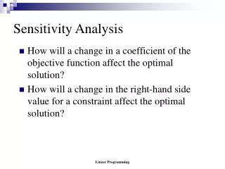
L INEAR PROGRAMMING SENSITIVITY ANALYSIS. Learning Objectives. Learn sensitivity concepts Understand, using graphs, impact of changes in objective function coefficients, right-hand-side values, and constraint coefficients on optimal solution of a linear programming problem.


L INEAR PROGRAMMING SENSITIVITY ANALYSIS
E N D
Presentation Transcript
Learning Objectives • Learn sensitivity concepts • Understand, using graphs, impact of changes in objective function coefficients, right-hand-side values, and constraint coefficients on optimal solution of a linear programming problem. • Generate answer and sensitivity reports using Excel's Solver. • Interpret all parameters of reports for maximization and minimization problems. • Analyze impact of simultaneous changes in input data values using 100% rule. • Analyze the impact of addition of new variable using pricing-out strategy.
Introduction (1 of 2) • Optimal solutions to LP problems have been examined under deterministic assumptions. • Conditions in most real world situations are dynamic and changing. • After an optimal solution to problem is found, input data values are varied to assess optimal solutionsensitivity. • This process is also referred to as sensitivity analysis or post-optimality analysis.
Introduction (2 of 2) • Sensitivity analysis determines the effect on optimal solutions of changes in parameter values of the objective function and constraint equations • Changes may be reactions to anticipated uncertainties in the parameters or the new or changed information concerning the model
The Role of Sensitivity Analysis of the Optimal Solution • Is the optimal solution sensitive to changes in input parameters? • Possible reasons for asking this question: • Parameter values used were only best estimates. • Dynamic environment may cause changes. • “What-if” analysis may provide economical and operational information.
1. Sensitivity Analysis of Objective Function Coefficients.
Ranges of Optimality • The optimal solution will remain unchanged as long as: • an objective function coefficient lies within its range of optimality • there are no changes in any other input parameters. The value of the objective function will change if the coefficient multiplies a variable whose value is nonzero.
Sensitivity Analysis Using GraphsExample 1: High Note Sound Company(HNSC) (1 of 4) • HNSC Manufactures quality CD players and stereo receivers. • Each product requires skilled craftsmanship. • LP problem formulation: Objective: maximize profit = $50C + $120R subject to 2C + 4R 80 (Hours of electricians' time available) 3C + R 60 (Hours of audio technicians' time available) C, R 0 (Non-negativity constraints) Where: C = number of CD players to make. R = number of receivers to make.
Sensitivity Analysis Using Graphs Example 1 (3 of 4) Impact of price change of Receivers If unit profit per stereo receiver (R) increased from $120 to $150, is corner point a still the optimal solution? YES ! But Profit is$3,000 = 0 ($50) + 20 ($150)
Sensitivity Analysis Using GraphsExample 1 (4 of4) Impact of price change of Receivers If receiver’s profit coefficient changed from $120 to $80, slope of isoprofit line changes causing corner point (b) to become optimal. But Profit is $1,760 = 16 ($50) + 12 ($80).
Sensitivity Analysis Using GraphsExample 2: Galaxy Industries (1 of 5) Max 8X1 + 5X2 (Weekly profit) subject to 2X1 + 1X2 < = 1200 (Plastic) 3X1 + 4X2 < = 2400 (Production Time) X1 + X2 < = 800 (Total production) X1 - X2 < = 450 (Mix) Xj> = 0, j = 1,2 (Nonnegativity)
Sensitivity Analysis Using Graphs Example 2:(2 of 5) Profit = $ 000 Recall the feasible Region We now demonstrate the search for an optimal solution Start at some arbitrary profit, say profit = $2,000... X2 1200 Then increase the profit, if possible... ...and continue until it becomes infeasible Profit =$5040 4, 2, 3, 800 600 X1 400 600 800
Sensitivity Analysis Using GraphsExample 2 (3 of 5) MODEL SOLUTION Space Rays = 480 dozens Zappers = 240 dozens Profit = $5040 • This solution utilizes all the plastic and all the production hours. • Total production is only 720 (not 800). • Space Rays production exceeds Zapper by only 240 dozens (not 450).
Sensitivity Analysis Using GraphsExample 2 (4 of 5) X2 1200 The effects of changes in an objective function coefficient on the optimal solution 800 Max 8x1 + 5x2 600 Max 4x1 + 5x2 Max 3.75x1 + 5x2 Max 2x1 + 5x2 X1 400 600 800
Range of optimality Sensitivity Analysis Using GraphsExample 2 (5 of 5) X2 1200 Max8x1 + 5x2 10 Max 10 x1 + 5x2 Max 3.75 x1 + 5x2 3.75 800 600 Max8x1 + 5x2 Max 3.75x1 + 5x2 X1 400 600 800 The effects of changes in an objective function coefficients on the optimal solution
The optimality range for an objective coefficient is the range of values over which the current optimal solution point will remain optimal
For two variable LP problems the optimality ranges of objective function coefficients can be found by setting the slope of the objective function equal to the slopes of each of the binding constraints
Sensitivity Analysis Using Graphs Example 3: Beaver Creek Pottery (1 of 4) Maximize Z = $40x1 + $50x2 subject to: 1x1 + 2x2 40 4x2 + 3x2 120 x1, x2 0
Sensitivity Analysis Using Graphs Example 3 (2 of 4) Maximize Z = $100x1 + $50x2 subject to: 1x1 + 2x2 40 4x2 + 3x2 120 x1, x2 0
Sensitivity Analysis Using Graphs Example 3 (3 of 4) Maximize Z = $40x1 + $100x2 subject to: 1x1 + 2x2 40 4x2 + 3x2 120 x1, x2 0
Objective Function Coefficient Sensitivity Range • The sensitivity range for an objective function coefficient is the range of values over which the current optimal solution point will remain optimal. • The sensitivity range for the xi coefficient is designated as ci.
Objective Function CoefficientSensitivity Range for c1 and c2Example 3 (4 of 4) objective function Z = $40x1 + $50x2 sensitivity range for: x1: 25 c1 66.67 x2: 30 c2 80
Objective Function Coefficient Sensitivity Range (for a Cost Minimization Model) Minimize Z = $6x1 + $3x2 subject to: 2x1 + 4x2 16 4x1 + 3x2 24 x1, x2 0 sensitivity ranges: 4 c1 0 c2 4.5
Multiple changes • The range of optimality is valid only when a single objective function coefficients changes. • When more than one variable changes we turn to the 100% rule.
The 100% Rule 1. For each increase (decrease) in an objective function coefficient, calculate (and express as a percentage) the ratio of the change in the coefficient to the maximum possible increase (decrease) as determined by the limits of the range of optimality. 2. Sum all these percent changes. If the total is less than 100 percent, the optimal solution will not change. If this total is greater than or equal to 100%, the optimal solution may change.
Reduced Costs The reduced cost for a variable at its lower bound (usually zero) yields: • The amount the profit coefficient must change before the variable can take on a value above its lower bound. • The amount the optimal profit will change per unit increase in the variable from its lower bound.
Changes in Right-Hand-Side Values of Constraints The sensitivity range for a RHS value is the range of values over which the quantity (RHS) values can change without changing the solution variable mix, including slack variables.
Sensitivity Analysis of Right-Hand SideValues • Any change in the right hand side of a binding constraint will change the optimal solution. • Any change in the right-hand side of a nonbinding constraint that is less than its slack or surplus, will cause no change in the optimal solution.
Changes in Constraint Quantity (RHS) Values Increasing the Labor Constraint (1 of 3) Example 1: Beaver Creek Maximize Z = $40x1 + $50x2 subject to: 1x1 + 2x2 40 4x2 + 3x2 120 x1, x2 0
Changes in Constraint Quantity (RHS) Values Sensitivity Range for Labor Constraint (2 of 3) Example 1: Beaver Creek Sensitivity range for: 30 q1 80 hr
Changes in Constraint Quantity (RHS) Values Sensitivity Range for Clay Constraint (3 of 3) Example 1: Beaver Creek Sensitivity range for: 60 q2 160 lb
Sensitivity Analysis of Right-Hand SideValues & Shadow Prices In sensitivity analysis of right-hand sides of constraints we are interested in the following questions: • Keeping all other factors the same, how much would the optimal value of the objective function (for example, the profit) change if the right-hand side of a constraint is changed by one unit? • For how many additional or fewer units this per unit this change will be valid?
Changes in Right-hand-side (RHS) & Shadow Prices RHS of Binding Constraint - • If RHS of non-redundant constraint changes, size of feasible region changes. • If size of region increases, optimal objective function improves. • If size of region decreases, optimal objective function worsens. • Relationship expressed as Shadow Price. • Shadow Price is change in optimal objective function value for one unit increase in RHS.
Shadow Prices (Dual Values) • Defined as the marginal value of one additional unit of resource. • The sensitivity range for a constraint quantity value is also the range over which the shadow price is valid.
Range of Feasibility • The set of right - hand side values for which same set of constraints determines the optimal point. • Within the range of feasibility, shadow prices remain constant; however, the optimal solution will change.
Example 2: High Note Sound Company Problem (1 of 6) • HNSC Manufactures quality CD players and stereo receivers. • Each product requires skilled craftsmanship. • LP problem formulation: Objective: maximize profit = $50C + $120R subject to 2C + 4R 80 (Hours of electricians' time available) 3C + R 60 (Hours of audio technicians' time available) C, R 0 (Non-negativity constraints) Where: C = number of CD players to make. R = number of receivers to make.
Sensitivity Analysis of Right-hand-side (RHS) ValuesExample 2: High Note Sound Company (2 of 6) May change the feasible region size. May change or move corner points.
Increase in Electricians’ Available TimeExample2: High Note Sound Company (3 of 6) • As available electricians’ time increases, corner points a and b will move closer to one other. • Further increases in available electricians’ time may make this constraint redundant.
Decrease in Electricians’ Available TimeExample 2: High Note Sound Company (4 of 6) • As available electricians’ time decreases, corner points b and c move closer to one another from their current locations. • Corner points b and c will no longer be feasible, and intersection of electricians’ time constraint with horizontal (C) axis will become a new feasible corner point.
Primary information is provided by Shadow Price • Resources available: • 80 hours of electricians’ time. • 60 hours of audio technicians’ time. • Final Values in table reveal optimal solution requires: • all 80 hours of electricians’ time. • Only 20 hours of audio technicians’ time. • Electricians’ time constraint is binding. • Audio technicians’ time constraint is non-binding. • 40 unused hours of audio technicians’ time are referred to as slack.
Changes in Right-Hand-Side (RHS) Example 2: High Note Sound Company (5 of 6) • In case of electrician hours Shadow Price is $30. • For each additional hour of electrician time thatfirm can increase profits by $30.
Changes in RHS of a Non-binding ConstraintExample 2: High Note Sound Company (6 of 6) • Audio technicians’ time has 40 unused hours. • No interest in acquiring additional hours of resource. • Shadow price for audio technicians’ time is zero. • Once 40 hours is lost (current unused portion, or slack) of audio technicians’ time, resource also becomes binding. • Any additional loss of time will clearly have adverse effect on profit. • Reduced Cost value - shows amount one will ‘lose’ ifsolution is forced to make an additional unit.
Sensitivity Analysis For A Larger Maximization Example Example 3: Anderson Electronics (1 of 8) Considering producing four potential products: VCRs, stereos, televisions (TVs), and DVD players: Profit per unit: VCR Stereo TV DVD $41 $32 $72 $54
LP FormulationExample 3: Anderson Electronics(2 of 8) Objective: maximize profit = $29 V + $32 S + $72 T + $54 D subject to 3 V + 4 S + 4 T + 3 D 4700 (Electronic components) 2 V + 2 S + 4 T + 3 D 4500 (Non-electronic components) 1 V + 1 S + 3 T + 2 D 2500 (Assembly time in hours) V, S, T, D 0 Where: V = number of VCRs to produce. S = number of Stereos to produce. T = number of TVs to produce. D = number of DVD players to produce.
Excel Solver Sensitivity ReportExample 3: Anderson Electronics (3 of 8) Non Zero value decision variables, Stereos and DVDs: Produce 380 Stereos with unit profit of $32. • Decision should not change as profit is between $31.33 and $72: Produce 1060 DVDs with unit profit of $54. • Decision should not change as profit is between $49 and $64:
Example 3: Anderson Electronics (4 of 8) Zero value decision variables, VCRs and TVs: Produce 0 VCRs (Reduced cost of $1.00) • Decision to make 0 should not change as profit is below $29 – but should change over and $30: Produce 0 TVs with unit cost of$8.00 (Reduced Cost). • Decision to make 0 should not change as profit is below $72 – but should change over and $80:
Simultaneous Changes In Parameter ValuesExample 3: Anderson Electronics (5 of 8) Possible to analyze impact of simultaneous changes on optimal solution only under specific condition: • (Change / Allowable change) 1 • If decrease RHS from 4,700 to 4,200, allowable decrease is 950. The ratio is: 500 / 950 = 0.5263 • If increase 200 hours (from 2,500 to 2,700) in assembly time, allowable increase is 466.67. The ratio is: 200 / 466.67 = 0.4285 • The sum of these ratios is: Sum of ratios = 0.5263 + 0.4285 = 0.9548 < 1 Since sum does not exceed 1, information provided in sensitivity report is valid to analyze impact of changes.
Simultaneous Changes In Parameter Values Example 3:Anderson Electronics (6 of 8) • Decrease of 500 units in electronic component availability reduces size of feasible region and causes profit to decrease. • Magnitude of decrease is $1,000 (500 units x $2 per unit). • Increase of 200 hours of assembly time results in larger feasible region and net increase in profit. • Magnitude of increase is $4,800 (200 hours x $24 per hour). • Net impact of both changes simultaneously is an increase in profit by $3,800 ( $4,800 - $1,000).