LINEAR PROGRAMMING Introduction to Sensitivity Analysis
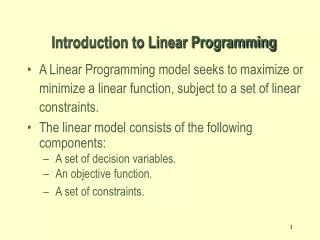
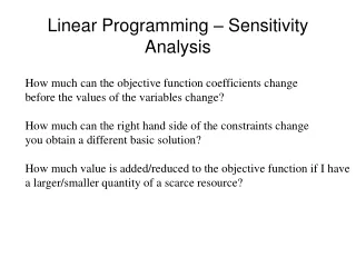
Learn how changes in coefficients, RHS values, and constraint coefficients impact optimal solutions in linear programming. Use Excel's Solver to generate and interpret sensitivity reports for maximization and minimization problems. Explore the range of optimality, shadow prices, and software output details.

LINEAR PROGRAMMING Introduction to Sensitivity Analysis
E N D
Presentation Transcript
LINEAR PROGRAMMING Introduction to Sensitivity Analysis Professor Ahmadi
Learning Objectives • Understand, using graphs, impact of changes in objective function coefficients, right-hand-side values, and constraint coefficients on optimal solution of a linear programming problem. • Generate answer and sensitivity reports using Excel's Solver. • Interpret all parameters of reports for maximization and minimization problems. • Analyze impact of simultaneous changes in input data values using 100% rule.
Sensitivity Analysis • Sensitivity analysis (or post-optimality analysis) is used to determine how the optimal solution is affected by changes, within specified ranges, in: • the objective function coefficients • the right-hand side (RHS) values • Sensitivity analysis is important to the manager who must operate in a dynamic environment with imprecise estimates of the coefficients. • Sensitivity analysis allows the manager to ask certain what-if questions about the problem.
Range of Optimality: The Objective Function Coefficients • A range of optimality of an objective function coefficient is found by determining an interval for the coefficient in which the original optimal solution remains optimal while keeping all other data of the problem constant. (The value of the objective function may change in this range.)
The Right Hand Sides: Shadow Price (Dual Price) • A shadow price for a right hand side value (or resource limit) is the amount the objective function will change per unit increase in the right hand side value of a constraint. • The range of feasibility for a change in the right hand side value is the range of values for this coefficient in which the original shadow price remains constant. • Graphically, a shadow price is determined by adding +1 to the right hand side value in question and then resolving for the optimal solution in terms of the same two binding constraints. • The shadow price is equal to the difference in the values of the objective functions between the new and original problems. • The shadow price for a non-binding constraint is 0.
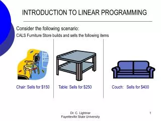
Example 1 • Refer to the “Woodworking” example of Chapter 2, where X1 = Tables and X2= Chairs. The problem is shown below. Max. Z= $100X1+60X2 s.t. 12X1+4X2 < 60 (Assembly time in hours) 4X1+8X2 < 40 (Painting time in hours) The optimum solution was X1=4, X2=3, and Z=$580. Answer the following questions regarding this problem.
Answer the following Questions: 1. Compute therange of optimalityfor the contribution of X1 (Tables) 2. Compute therange of optimalityfor the contribution of X2 (Chairs) 3. Determine thedual Price (Shadow Price) for the assembly stage. 4. Determine thedual Price (Shadow Price) for the painting stage.
Standard Computer Output • Software packages such as Microsoft Excel and LINDO provide the following LP information: • Information about the objective function: • its optimal value • coefficient ranges (ranges of optimality) • Information about the decision variables: • their optimal values • their reduced costs • Information about the constraints: • the amount of slack or surplus • the dual prices • right-hand side ranges (ranges of feasibility)
Sensitivity Report • Sensitivity report has two distinct components. • (1) Table titled Adjustable Cells • (2) Table titled Constraints. • Tables permit one to answer several "what-if" questions regarding problem solution. • Consider a change to only a single input data value. • Sensitivity information does not always apply to simultaneous changes in several input data values.
Example 2: Olympic Bike Co. • Model Formulation Max 10x1 + 15x2 (Total Weekly Profit) s.t. 2x1 + 4x2 < 100 (Aluminum Available) 3x1 + 2x2 < 80 (Steel Available) x1, x2 > 0 (Non-negativity)
Example 2: Olympic Bike Co. • Optimal Solution According to the output: x1 (Deluxe frames) = 15, x2 (Professional frames) = 17.5, and the objective function value = $412.50.
Example 2: Olympic Bike Co. • Range of Optimality Question Suppose the profit on deluxe frames is increased to $20. Is the above solution still optimal? What is the value of the objective function when this unit profit is increased to $20? Answer The output states that the solution remains optimal as long as the objective function coefficient of x1 is between 7.5 and 22.5. Since 20 is within this range, the optimal solution will not change. The optimal profit will change: 20x1 + 15x2 = 20(15) + 15(17.5) = $562.50
Example 2: Olympic Bike Co. • Range of Optimality Question If the unit profit on deluxe frames were $6 instead of $10 would the optimal solution change? Answer The output states that the solution remains optimal as long as the objective function coefficient of x1 is between 7.5 and 22.5. Since 6 is outside this range, the optimal solution would change.
Example 2: Olympic Bike Co. • Range of Feasibility: The range of feasibility for a change in a right-hand side value is the range of values for this parameter in which the original shadow price remains constant. Question What is the maximum amount the company should pay for 50 extra pounds of aluminum? Answer The shadow price provides the value of extra aluminum. The shadow price for aluminum is $3.125 per pound and the maximum allowable increase is 60 pounds. Since 50 is in this range, then the $3.125 is valid. Thus, the value of 50 additional pounds is: 50($3.125) = $156.25
Example 3 • Consider the following linear program: Min 6x1 + 9x2 ($ cost) s.t. x1 + 2x2 < 8 10x1 + 7.5x2 > 30 x2 > 2 x1, x2> 0 Solve the above problem and perform sensitivity analysis.
Range of Optimality and 100% Rule • The 100% rule states that simultaneous changes in objective function coefficients will not change the optimal solution as long as the sum of the percentages of the change divided by the corresponding maximum allowable change in the range of optimality for each coefficient does not exceed 100%.
Range of Feasibility • A dual price represents the improvement (increase or decrease) in the objective function value per unit increase in the right-hand side. As long as the right-hand side remain within the range of feasibility, there will be is no change in the shadow price. The range of feasibility is the range over which the dual price is applicable.
Range of Feasibility and 100% Rule • The 100% rule states that simultaneous changes in right-hand sides will not change the dual prices as long as the sum of the percentages of the changes divided by the corresponding maximum allowable change in the range of feasibility for each right-hand side does not exceed 100%.
Reduced Cost • The reduced cost for a decision variable whose value is 0 in the optimal solution is the amount the variable's objective function coefficient would have to improve (increase for maximization problems, decrease for minimization problems) before this variable could assume a positive value. • The reduced cost for a decision variable with a positive value is 0.
Example 4 In a product-mix-problem, X1, X2, X3, and X4 indicate the units of products 1, 2, 3, and 4, respectively, and the linear programming model is MAX Z = $5X1+$7X2+$8X3+$6X4 S.T. 1) 3X1+2X2+4X3+3X4600 Machine A hours 2) 4X1+1X2+2X3+6X4700 Machine B hours 3) 2X1+3X2+1X3+2X4800 Machine C hours Input the data in an Excel file and save the file. Using Solver, solve the problem and obtain sensitivity results.
Summary • Sensitivity analysis used by management to answer series of “ what-if ” questions about LP model inputs. • Tests sensitivity of optimal solution to changes: • Profit or cost coefficients, and • Constraint RHS values. • Explored sensitivity analysis graphically (with two decision variables). • Discussed interpretation of information: • In answer and sensitivity reports generated by Solver. • In reports used to analyze simultaneous changes in model parameter values.