Lower resolution X-ray spectroscopy
370 likes | 403 Views
Understand the basics of X-ray spectroscopy, analysis methods, energy calculations, and spectral fitting techniques. Learn about instruments like ROSAT PSPC and Chandra ACIS. Explore the challenges of interpreting X-ray spectra in comparison to optical data.

Lower resolution X-ray spectroscopy
E N D
Presentation Transcript
Lower resolution X-ray spectroscopy Keith Arnaud NASA Goddard University of Maryland X-ray School 2003
Practical X-ray spectroscopy Most X-ray spectra are of moderate or low resolution (eg Chandra ACIS or XMM-Newton EPIC). However, the spectra generally cover a bandpass of more than 1.5 decades in energy. Moreover, the continuum shape often provides important physical information. Therefore, unlike in the optical, most uses of X-ray spectra have involved a simultaneous analysis of the entire spectrum rather than an attempt to measure individual line strengths. X-ray School 2003
Martin Elvis Proportional counter e.g. ROSAT PSPC 3C 273 Optical Spectrum CCD e.g. Chandra ACIS Grating X-ray School 2003
Can we start with these… and deduce this ? X-ray School 2003
Can we start with this… X-ray School 2003
and deduce this X-ray School 2003
The Basic Problem Suppose we observe D(I) counts in channel I (of N) from some source. Then : D(I) = T ∫ R(I,E) A(E) S(E) dE • T is the observation length (in seconds) • R(I,E) is the probability of an incoming photon of energy E being registered in channel I (dimensionless) • A(E) is the energy-dependent effective area of the telescope and detector system (in cm2) • S(E) is the source flux at the front of the telescope (in photons/cm2/s/keV X-ray School 2003
An example R(I,E) photopeak photopeak fluorescence fluourescence escape escape X-ray School 2003
Example A(E) X-ray School 2003
Analogs in optical/UV An example R(I,E) would be the resolution of a spectrometer. In most optical/UV instruments R(I,E) is simple - a Gaussian or Lorentzian shape. A(E) is the product of telescope reflectivities, detector efficiencies, and filter transmissions. In optical/UV astronomy we usually divide the observed data by this function to obtain the fluxed spectrum. X-ray School 2003
But can I ignore the response ? Sometimes, yes. If you have CCD (eg Chandra ACIS or XMM-Newton EPIC) spectra you must use the response, R(I,E). If you have Chandra HETG spectra then you can treat them like optical/UV spectra. However, for XMM-Newton RGS if you try to do this you will get incorrect results. The RGS spectral response has wide wings so line fluxes will be wrong and the continuum level overestimated. X-ray School 2003
The Basic Problem II D(I) = T ∫ R(I,E) A(E) S(E) dE We assume that T, A(E) and R(I,E) are known and want to solve this integral equation for S(E). We can divide the energy range of interest into M bins and turn this into a matrix equation : Di= T ∑Rij Aj Sj where Sj is now the flux in photons/cm2/s in energy bin J. We want to find Sj. X-ray School 2003
The Basic Problem III Di = T ∑Rij Aj Sj The obvious tempting solution is to calculate the inverse of Rij, premultiply both sides and rearrange : (1/T Aj) ∑(Rij)-1Di = Sj This does not work ! The Sj derived in this way are very sensitive to slight changes in the data Di. This is a great method for amplifying noise. X-ray School 2003
A (brief) Mathematical Digression This should not have come as a surprise to anyone with any data analysis experience. This is the “remote sensing problem” and arises in many areas of astronomy as well as eg geophysics and medical imaging. In mathematics the integral is known as a Fredholm equation of the first kind. Tikhonov showed that such equations can be solved using “regularization” - applying prior knowledge to damp the noise. A familiar example is maximum entropy but there are a host of others. Some of these have been tried on X-ray spectra - none have had any impact on the field. X-ray School 2003
Forward-fitting • The standard method of analyzing X-ray spectra is “forward-fitting”. This comprises the following steps… • Calculate a model spectrum. • Multiply the result by an instrumental response matrix (R(I,E)*A(E)). • Compare the result with the actual observed data by calculating some statistic. • Modify the model spectrum and repeat till the best value of the statistic is obtained. X-ray School 2003
Define Model Forward-fitting algorithm Calculate Model Multiply by detector response Change model parameters Compare to data X-ray School 2003
This only works if the model spectrum can be expressed in a reasonably small number of parameters (although I have seen people fit spectra using models with over 100 parameters). The aim of the forward-fitting is then to obtain the best-fit and confidence ranges of these parameters. X-ray School 2003
Spectral fitting programs • XSPEC- part of HEAsoft. General spectral fitting program with many models available. • Sherpa - part of CIAO. Multi-dimensional fitting program which includes the XSPEC model library and can be used for spectral fitting. • SPEX - from SRON in the Netherlands. Spectral fitting program specialising in collisional plasmas and high resolution spectroscopy. • ISIS - from the MIT Chandra HETG group. Mainly intended for the analysis of grating data. Incorporated in Sherpa as GUIDE. X-ray School 2003
Models All models are wrong, but some are useful - George Box X-ray spectroscopic models are usually built up from individual components. These can be thought of as two basic types -additive (an emission component e.g. blackbody, line,…) or multiplicative (something which modifies the spectrum e.g. absorption). Model = M1 * M2 * (A1 + A2 + M3*A3) + A4 X-ray School 2003
XSPEC>model ? Possible additive models are : apec bbody bbodyrad bexrav bexriv bknpower bkn2pow bmc bremss c6mekl c6pmekl c6pvmkl c6vmekl cemekl cevmkl cflow compbb compLS compST compTT cutoffpl disk diskbb diskline diskm disko diskpn equil gaussian gnei grad grbm laor lorentz meka mekal mkcflow nei npshock nteea pegpwrlw pexrav pexriv photoion plcabs powerlaw posm pshock raymond redge refsch sedov srcut sresc step vapec vbremss vequil vgnei vmeka vmekal vmcflow vnei vnpshock vpshock vraymond vsedov zbbody zbremss zgauss zpowerlw atable Possible multiplicative models are : absori acisabs constant cabs cyclabs dust edge expabs expfac highecut hrefl notch pcfabs phabs plabs pwab redden smedge spline SSS_ice TBabs TBgrain TBvarabs uvred varabs vphabs wabs wndabs xion zedge zhighect zpcfabs zphabs zTBabs zvarabs zvfeabs zvphabs zwabs zwndabs mtable etable Possible mixing models are : ascac projct xmmc Possible convolution models are : gsmooth lsmooth reflect rgsxsrc Possible pile-up models are : pileup X-ray School 2003
Additive Models • Basic additive (emission) models include : • blackbody • thermal bremsstrahlung • power-law • collisional plasma (raymond, mekal, apec) • Gaussian or Lorentzian lines • There are many more models available covering specialised topics such as accretion disks, comptonized plasmas, non-equilibrium ionization plasmas, multi-temperature collisional plasmas… X-ray School 2003
Multiplicative Models • and multiplicative models include : • photoelectric absorption due to our Galaxy • photoelectric absorption due to ionized material • high energy exponential roll-off. • cyclotron absorption lines. X-ray School 2003
Galactic absorption X-ray School 2003
Convolution Models(for the aficionados) • These are models which take as input the current model and manipulate it in some way. Examples are : • Smoothing with a Gaussian or Lorentzian function (e.g. velocity broadening) • Compton reflection • Pile-up X-ray School 2003
Roll Your Own Models There is a simple XSPEC model interface which enables astronomers to write new models and fit them to their data. You can write your own subroutine (in Fortran or C) and hook it in - the subroutine takes in the energies on which to calculate the model and writes out the fluxes (in photons/cm2/s). In addition, there is also a standard format for files containing model spectra so these too can be fit to data without having to add new routines to XSPEC. X-ray School 2003
Finding the best-fit Finding the best-fit means minimizing the statistic value. There are many algorithms available to do this in a computationally efficient fashion (see Numerical Recipes). Most methods used to find the best-fit are local i.e. they use some information around the current parameters to guess a new set of parameters. All these methods are liable to get stuck in a local minimum. Watch out for this ! X-ray School 2003
Finding the best-fit Finding the best-fit means minimizing the statistic value. There are many algorithms available to do this in a computationally efficient fashion (see Numerical Recipes). Most methods used to find the best-fit are local i.e. they use some information around the current parameters to guess a new set of parameters. All these methods are liable to get stuck in a local minimum. Watch out for this ! The more complicated your model and the more highly correlated the parameters then the more likely that the algorithm will not find the absolute best-fit. X-ray School 2003
Finding the best-fit II Sometimes you can spot that you are stuck in a local minimum by using the XSPEC error or steppar commands. These both step through parameter values, error in the vicinity of the current best-fit and steppar over a user-defined grid, and thus can stumble across a better fit. Crude but sometimes effective. You can do this in a semi-automated fashion by using a local minimization algorithm and following this with the error command with the ability to restart if a new minimum is found during the search. X-ray School 2003
Global Minimization There are global minimization methods available - simulated annealing, genetic algorithms, … - but they require many function evaluations (so are slow) and are still not guaranteed to find the true minimum. A new technique called Markov Chain Monte Carlo, which provides an intelligent sampling of parameter space, looks promising but it is not yet widely available (i.e. I’ve not added it to XSPEC - yet). X-ray School 2003
Dealing with background • Unless you are looking at a bright point source with Chandra you will probably have a background component to the spectrum in addition to the source in which you are interested. • You can include background in the model but this is complicated and is not usually used. • The usual method is to extract a spectrum from another part of the image or another observation. Spectral fitting programs then use both the source and background spectra. • If the background spectrum is extracted from a different sized region than the source then the background spectrum is scaled by the spectral fitting program (using the BACKSCAL keyword in the FITS file). X-ray School 2003
Spectra with few counts • Be careful if you have few photons/bin. Chi-squared is biased in this case with fluctuations below the model having more weight than those above, causing the fit model to lie below the true model. • A common solution is to bin up your spectrum so all the bins have > some number of photons. Don’t do this - it loses information and introduces a bias that is difficult to quantify. • Solutions are to use a different weighting scheme (I prefer the weight churazov option in XSPEC) or a maximum likelihood statistic (the “C statistic” - stat cstat in XSPEC). • The problem with these options is that while they give best fit parameters they do not provide a goodness-of-fit measure. X-ray School 2003
Final Advice and Admonitions • Remember that the purpose of spectral fitting is to attain understanding, not fill up tables of numbers. • Don’t bin up your data - especially in a way that is dependent on the data values (eg group min 15). • Don’t misuse the F-test. • Try to test whether you really have found the best-fit. X-ray School 2003