Download
1 / 40
570 likes | 1.23k Views
Robust Control Systems (Chapter 12).

E N D
Robust Control Systems (Chapter 12) Feedback control systems are widely used in manufacturing, mining, automobile and other hardware applications. In response to increased demands for increased efficiency and reliability, these control systems are being required to deliver more accurate and better overall performance in the face of difficult and changing operating conditions. In order to design control systems to meet the needs of improved performance and robustness when controlling complicated processes, control engineers will require new design tools and better control theory. A standard technique of improving the performance of a control system is to add extra sensors and actuators. This necessarily leads to a multi-input multi-output (MIMO) control system. Accordingly, it is a requirement for any modern feedback control system design methodology that it be able to handle the case of multiple actuators and sensors. Robust means durable, hardy, and resilient
Why Robust? • When we design a control system, our ultimate goal is to control a particular system in a real environment. • When we design the control system we make numerous assumptions about the system and then we describe the system with some sort of mathematical model. • Using a mathematical model permits us to make predictions about how the system will behave, and we can use any number of simulation tools and analytical techniques to make those predictions. • Any model incorporates two important problems that are often encountered: a disturbance signal is added to the control input to the plant. That can account for wind gusts in airplanes, changes in ambient temperature in ovens, etc., and noise that is added to the sensor output.
+ Prefilter GP(s) Controller GC(s) Plant G(s) + Y(s) Output + - + Sensor 1 + N(s) Noise A robust control system exhibits the desired performance despite the presence of significant plant (process) uncertaintyThe goal of robust design is to retain assurance of system performance in spite of model inaccuracies and changes. A system is robust when it has acceptable changes in performance due to model changes or inaccuracies. D(s) Disturbance R(s)
Why Feedback Control Systems? • Decrease in the sensitivity of the system to variation in the parameters of the process G(s). • Ease of control and adjustment of the transient response of the system. • Improvement in the rejection of the disturbance and noise signals within the system. • Improvement in the reduction of the steady-state error of the system
Sensitivity of Control Systems to Parameter Variations • A process, represented by G(s), whatever its nature, is subject to a changing environment, aging, ignorance of the exact values of the process parameters, and the natural factors that affect a control process. • The sensitivity of a control system to parameter variations is very important. A main advantage of a closed-loop feedback system is its ability to reduce the system’s sensitivity. • The system sensitivity is defined as the ratio of the percentage change in the system transfer function to the percentage change of the process transfer function.
The sensitivity of the feedback system to changes in the feedback element H(s) is
1/s+ + Y(s) R(s) - Robust Control Systems and System SensitivityA control system is robust when: it has low sensitivities, (2) it is stable over the range of parameter variations, and (3) the performance continues to meet the specifications in the presence of a set of changes in the system parameters.
K/s(s+1) + Y(s) R(s) - Let us examine the sensitivity of the following second-order system
Example 12.1: Sensitivity of a Controlled System GC(s) G(s) + R(s) Y(s) Controller b1+b2s Plant 1/s2 -
Bode PlotFrequency response plots of linear systems are often displayed in the form of logarithmic plots, called Bode plots, where the horizontal axis represents the frequency on a logarithmic scale (base 10) and the vertical axis represents the amplitude ratio or phase of the frequency response function.
Disturbance Signals in a Feedback Control System • Another important effect of feedback in a control system is the control and partial elimination of the effect of disturbance signal. • A disturbance signal is an unwanted input signal that affects the system output signal. Electronic amplifiers have inherent noise generated within the integrated circuits or transistors; radar systems are subjected to wind gusts; and many systems generate all kinds of unwanted signals due to nonlinear elements. • Feedback systems have the beneficial aspects that the effect of distortion, noise, and unwanted disturbances can be effectively reduced.
The Steady-State Error of a Unity Feedback Control System (5.7) • One of the advantages of the feedback system is the reduction of the steady-state error of the system. • The steady-state error of the closed loop system is usually several orders of magnitude smaller than the error of the open-loop system. • The system actuating signal, which is a measure of the system error, is denoted as Ea(s). Ea(s) G(s) Y(s) R(s) H(s)
Compensator • A feedback control system that provides an optimum performance without any necessary adjustments is rare. Usually it is important to compromise among the many conflicting and demanding specifications and to adjust the system parameters to provide suitable and acceptable performance when it is not possible to obtain all the desired specifications. • The alteration or adjustments of a control system in order to provide a suitable performance is called compensation. • A compensator is an additional component or circuit that is inserted into control system to compensate for a deficient performance. • The transfer function of a compensator is designated as GC(s) and the compensator may be placed in a suitable location within the structure of the system.
Root Locus Method • The root locus is a powerful tool for designing and analyzing feedback control systems. • It is possible to use root locus methods for design when two or three parameters vary. This provides us with the opportunity to design feedback systems with two or three adjustable parameters. For example the PID controller has three adjustable parameters. • The root locus is the path of the roots of the characteristic equation traced out in the s-plane as a system parameter is changed. • Read Table 7.2 to understand steps of the root locus procedure. • The design by the root locus method is based on reshaping the root locus of the system by adding poles and zeros to the system open loop transfer function and forcing the root loci to pass through desired closed-loop poles in the s-plane.
Example z1=-3+j1 Y(s) R(s) Controller GC(s) Plant G(s) + - j2 -z1 j1 -2 -1 -z1
+ Prefilter GP(s) Controller GC(s) Plant G(s) + Y(s) Output + - + Sensor 1 + N(s) Noise Analysis of Robustness
The Design of Robust Control Systems • The design of robust control systems is based on two tasks: determining the structure of the controller and adjusting the controller’s parameters to give an optimal system performance. This design process is done with complete knowledge of the plant. The structure of the controller is chosen such that the system’s response can meet certain performance criteria. • One possible objective in the design of a control system is that the controlled system’s output should exactly reproduce its input. That is the system’s transfer function should be unity. It means the system should be presentable on a Bode gain versus frequency diagram with a 0-dB gain of infinite bandwidth and zero phase shift. Practically, this is not possible! • Setting the design of robust system requires us to find a proper compensator, GC(s) such that the closed-loop sensitivity is less than some tolerance value.
PID ControllersPID stands for Proportional, Integral, Derivative. One form of controller widely used in industrial process is called a three term, or PID controller. This controller has a transfer function: A proportional controller (Kp) will have the effect of reducing the rise time and will reduce, but never eliminate, the steady state error. An integral control (KI) will have the effect of eliminating the steady-state error, but it may make the transient response worse. A derivative control (KD) will have the effect of increasing the stability of the system, reducing the overshoot, and improving the transient response.
Proportional-Integral-Derivative (PID) Controller kp + u(t) e(t) ki/s + + kis
Time- and s-domain block diagram of closed loop system PID Controller u(t) System r(t) e(t) y(t) + R(s) E(s) U(s) Y(s) -
PID and Operational AmplifiersA large number of transfer functions may be implemented using operational amplifiers and passive elements in the input and feedback paths. Operational amplifiers are widely used in control systems to implement PID-type control algorithms needed.
Figure 8.5 Inverting amplifier
Figure 8.30 Op-amp Integrator
Figure 8.35 Op-amp Differentiator The operational differentiator performs the differentiation of the input signal. The current through the input capacitor is CSdvs(t)/dt. That is the output voltage is proportional to the derivative of the input voltage with respect to time, and Vo(t) = _RFCSdvs(t)/dt
Linear PID Controller Z2(s) C1 C2 R2 R1 Z1(s) vo(t) vs(t)
Tips for Designing a PID Controller When you are designing a PID controller for a given system, follow the following steps in order to obtain a desired response. • Obtain an open-loop response and determine what needs to be improved • Add a proportional control to improve the rise time • Add a derivative control to improve the overshoot • Add an integral control to eliminate the steady-state error • Adjust each of Kp, KI, and KD until you obtain a desired overall response. • It is not necessary to implement all three controllers (proportional, derivative, and integral) into a single system, if not needed. For example, if a PI controller gives a good enough response, then you do not need to implement derivative controller to the system.
The popularity of PID controllers may be attributed partly to their robust performance in a wide range of operation conditions and partly to their functional simplicity, which allows engineers to operate them in a simple manner.
Root LocusRoot locus begins at the poles and ends at the zeros. j 4 K3 increasing r1 z1 j 2 r2 -2 z1 r1
Design of Robust PID-Controlled SystemsThe selection of the three coefficients of PID controllers is basically a search problem in a three-dimensional space. Points in the search space correspond to different selections of a PID controller’s three parameters. By choosing different points of the parameter space, we can produce different step responses for a step input.The first design method uses the (integral of time multiplied by absolute error (ITAE) performance index in Section 5.9 and the optimum coefficients of Table 5.6 for a step input or Table 5.7 for a ramp input. Hence we select the three PID coefficients to minimize the ITAE performance index, which produces an excellent transient response to a step (see Figure 5.30c). The design procedure consists of the following three steps.
The Three Design Steps of Robust PID-Controlled System • Step 1: Select the n of the closed-loop system by specifying the settling time. • Step 2: Determine the three coefficients using the appropriate optimum equation (Table 5.6) and the n of step 1 to obtain GC(s). • Step 3: Determine a prefilter GP(s) so that the closed-loop system transfer function, T(s), does not have any zero, as required by Eq. (5.47)
Input Signals; Overshoot; Rise Time; Settling Time • Step: r(t) = AR(s) = A/s • Ramp: r(t) = AtR(s) = A/s2 • The performance of a system is measured usually in terms of step response. The swiftness of the response is measured by the rise time, Tr, and the peak time, Tp. • The settling time, Ts, is defined as the time required for the system to settle within a certain percentage of the input amplitude. • For a second-order system with a closed-loop damping constant, we seek to determine the time, Ts, for which the response remains within 2% of the final value. This occurs approximately when
D(s) + GP(s) GC(s) G(s) + E(s) U(s) + Y(s) - Example 12.8: Robust Control of Temperature Using PID Controller employing ITAE performance for a step input and a settling time of less than 0.5 seconds. R(s)
D(s) + GP(s) GC(s) G(s) + E(s) U(s) + Y(s) - E12.1: Using the ITAE performance method for step input, determine the required GC(t). Assume n = 20 for Table 5.6. Determine the step response with and without a prefilter GP(s) R(s)